I Created a Python Program to Find Strings on Google Maps (e.g,. “Finxter” in Budapest) : Gábor Madarász

April 01, 2023 April 01, 2023

I Created a Python Program to Find Strings on Google Maps (e.g,. “Finxter” in Budapest)
by: Gábor Madarász
blow post content copied from Be on the Right Side of Change
click here to view original post

Rate this post

No, ChatGPT really doesn’t help with this (yet…) but it did help me write the code snippet explanation (which I attached after each code output).

In my example, we will take a special route in Budapest, using one of the easiest to use library, gmplot.

We can create our maps directly in HTML code using its many methods.
To access some functions, you need a Google Maps API key.

I used Python’s built-in zip function to create the Lat – Lon coordinates, you can learn more about zip here:

Recommended: Python zip() Built-in Function

We can work with the following methods of the GoogleMapPlotter object, which I will describe in detail:

GoogleMapPlotter

from_geocode(location, zoom=10, apikey='')
draw(path_file)
get()
geocode(location, apikey='')
text(lat, lon, text, color='red')
marker(lat, lon, color='#FF0000', title=None, precision=6, label=None, **kwargs)
enable_marker_dropping(color, **kwargs)
directions
scatter
circle
plot
heatmap
ground_overlay
polygon
grid

Let’s go through the functions using “code snippets”:

Find a location by name (from_geocode)

With the geocode method of the GoogleMapPlotter object, we can display a given address and its neighbourhood on the map.

Parameters of the method: location (str), zoom (int), apikey (str)

After creating your map, you have two options, either save the HTML file (.draw()) or store it as a string (with .get()). I use the .draw() method, where the only parameter is the file to create and its path.

import gmplot
apikey = '' # (your API key here)
gmap = gmplot.GoogleMapPlotter.from_geocode('Budapest', apikey=apikey)
gmap.draw("budapest_map.html")

Result:

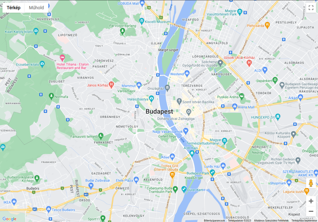
The code imports the gmplot library, which is a Python wrapper for the Google Maps API. It then creates a new GoogleMapPlotter object named gmap for the location “Budapest” using the from_geocode() method. This method uses the Google Maps API to retrieve the latitude and longitude of the location, which is necessary to display the map.

Finally, the draw() method is called on the gmap object to generate and save the map as an HTML file named budapest_map.html.

Coordinates of a location (geocode)

If you want to know the coordinates of a location, use .geocode(). As an input parameter, pass the name (str) of the place you are looking for and your API key. This returns a tuple of the lat/long coordinates of the given location (float, float).

import gmplot
apikey = '' # (your API key here)
location = gmplot.GoogleMapPlotter.geocode('Budapest, Hungary', apikey=apikey)
print(location)

Result:

(47.497912, 19.040235)

The code calls the geocode() method on the GoogleMapPlotter object to obtain the latitude and longitude of a location specified as a string. In this case, the location is “Budapest, Hungary”. The apikey parameter is also passed to this method to authenticate the Google Maps API.

Text on your map (text)

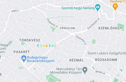
If you want to place custom text on your map, you can do it with .text(), using the text label’s Latitude and Longitude parameter.

It is possible to color the text with the color=str parameter, which can be the color name ('black'), hexadecimal ('#000000'), or matplotlib-like ('k').

import gmplot
apikey = ' ' # (your API key here)
gmap = gmplot.GoogleMapPlotter(47.519350864380385, 19.010462124312387, zoom = 17, apikey=apikey)
finxter_text = ['f', 'i', 'n', 'x', 't', 'e', 'r']
colors = ['limegreen', 'cyan', 'gold','orange', 'limegreen', 'cyan', 'orange']
j = 0
lat = 47.529266431577625
lng = 19.00500303401821
for i in finxter_text:
    gmap.text(lat, lng, i, color = colors[j])
    j += 1
    lng += 0.001

Result:

Drop marker (marker)

Show markers. The required parameters are, of course, the Latitude and Longitude coordinates (float, float), and additional optional parameters can be used to customize the markers:

color (str) which can be the name of the color ('black'), hexadecimal ('#000000'), or matplotlib-like ('k')
title (str) : Hover-over title of the marker.
precision (int) : Number of digits after the decimal to round to for lat/long values. Defaults to 6.
label (str) : Label displayed on the marker.
info_window (str) : HTML content to be displayed in a pop-up info window.
draggable (bool) : Whether or not the marker is draggable.

import gmplot
apikey = ' ' # (your API key here)
gmap.marker(47.51503432784726, 19.005350430919034, label = 'finxter', info_window = "<a href='https://finxter.com/'>The finxter Academy</a>", draggable = False)

gmap.enable_marker_dropping(color=’black’)

gmap.enable_marker_dropping() allows markers to be dropped onto the map when clicked. Clicking on a dropped marker will delete it.

Note: Calling this function multiple times will just overwrite the existing dropped marker settings.

Parameters:

color str: Color of the markers to be dropped.
title str: Hover-over title of the markers to be dropped.
label str: Label displayed on the markers to be dropped.
draggable bool: Whether or not the markers to be dropped are draggable.

Result:

The code adds a marker to the Google Maps plot. The marker is placed at the latitude and longitude coordinates (47.51503432784726, 19.005350430919034) and is labeled 'finxter'.

The info_window parameter sets the information displayed when the user clicks on the marker. In this case, it is a link to the Finxter Academy website.

The draggable parameter is set to False, meaning that the user cannot move the marker.

The fourth line enables marker dropping, meaning the user can add new markers to the plot by clicking on the map.

The final line saves the plot to an HTML file named marker.html.

Route planning (directions)

Using the Directions API, you can display route planning between any points. The origin and destination coordinates are given as parameters (float, float). Optionally, the waypoints as list of tuples and the travel_mode as str can also be specified. The travel modes are:

DRIVING (Default) indicates standard driving directions using the road network.
BICYCLING requests bicycling directions via bicycle paths & preferred streets.
TRANSIT requests directions via public transit routes.
WALKING requests walking directions via pedestrian paths & sidewalks.

import gmplot
apikey = ' ' # (your API key here)
gmap = gmplot.GoogleMapPlotter(47.519350864380385, 19.010462124312387, zoom = 14, apikey=apikey)
gmap.directions(
    (47.5194613766804, 19.000656008676216),
    (47.520243896650946, 19.00204002854648),
    waypoints = [(47.520888742275, 18.99871408933636)])
gmap.directions(
    (47.5194613766804, 19.000656008676216),
    (47.520243896650946, 19.00204002854648),
    waypoints = [(47.520888742275, 18.99871408933636)])

gmap.directions(
    (47.52226897515179, 19.00018393988221),
    (47.520243896650946, 19.00204002854648),
    waypoints = [(47.52088149688948, 19.002871513347902)])
gmap.draw('route.html')

Result:

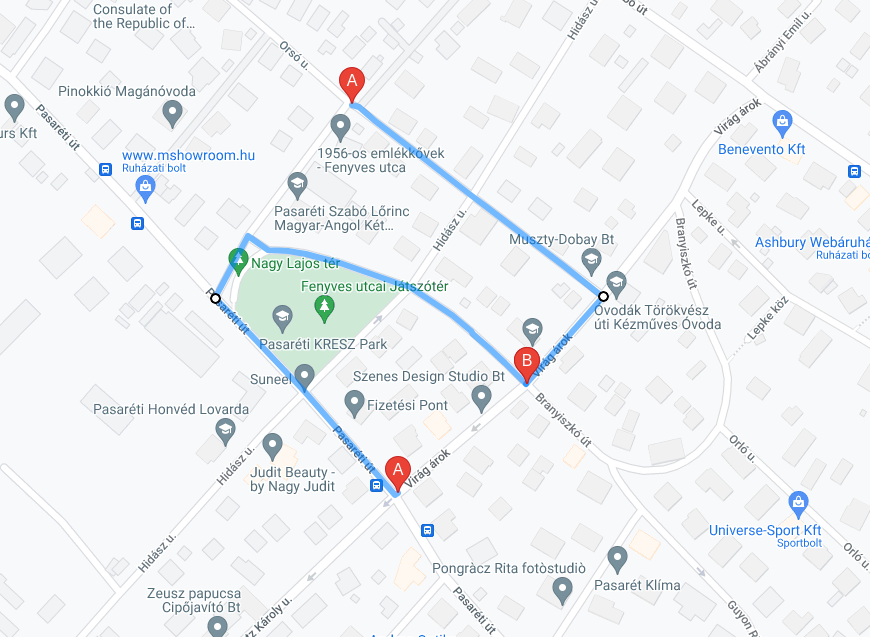
The fourth line adds a route to the plot using the directions() method.

The starting point of the route is at latitude 47.5194613766804 and longitude 19.000656008676216, and the ending point is at latitude 47.520243896650946 and longitude 19.00204002854648.

The waypoints parameter is set to a list containing one set of latitude and longitude coordinates (47.520888742275, 18.99871408933636).

The fifth line adds another route to the plot, starting at the same point as the previous route and ending at the same point as the previous route, but with different waypoints.

The sixth line adds a third route to the plot, with a starting point at latitude 47.52226897515179 and longitude 19.00018393988221, an ending point at latitude 47.520243896650946 and longitude 19.00204002854648, and a set of waypoints containing one set of latitude and longitude coordinates (47.52088149688948, 19.002871513347902).

Display many points (scatter)

The scatter() allows you to place many points at once. In addition to the necessary lat (float) and lon (float) parameters, the following optional parameters are:

color
size
marker
symbol
title
label
precision
face_alpha
edge_alpha
edge_width

import gmplot
apikey = ' ' # (your API key here)
gmap = gmplot.GoogleMapPlotter(47.519350864380385, 19.010462124312387, zoom = 14, apikey=apikey)
letters = zip(*[
    (47.51471253011692, 18.990678878050492),
    (47.51941514547201, 18.993554206158933),
    (47.52134244386804, 18.998060317311538),
    (47.52337110249922, 19.002008528961046),
    (47.52344355313603, 19.009969325319076),
    (47.52466070898612, 19.013488383565445),
    (47.526645771633746, 19.02031192332838)])
gmap.scatter(*letters,
    color=['limegreen', 'cyan','gold','orange', 'limegreen', 'cyan', 'orange'],
    s=60,
    ew=1,
    title=['f', 'i', 'n', 'x', 't', 'e', 'r'],
    label=['f', 'i', 'n', 'x', 't', 'e', 'r']
)
gmap.draw('scatter.html')

Result:

The fourth line defines a list of latitude and longitude coordinates as tuples, representing the locations of individual letters of the word 'finxter'.

The fifth line uses the scatter() method of adding the letters to the plot as points. The scatter() method takes the latitude and longitude coordinates as separate arguments using the unpacking operator (*letters).

The color parameter is set to a list of colors that correspond to the letters. The s parameter specifies the size of the points, the ew parameter specifies the width of the edge around the points, and the title and label parameters specify the title and label of each point, respectively.

Draw circle (circle)

Sometimes it is useful to draw a circle. In addition to specifying the center lat, lng, and radius of the circle, you can also to specify the following:

edge_alpha/ea float: Opacity of the circle’s edge, ranging from 0 to 1. Defaults to 1.0.
edge_width/ew int: Width of the circle’s edge, in pixels. Defaults to 1.
face_alpha/alpha float: Opacity of the circle’s face, ranging from 0 to 1. Defaults to 0.5.
color/c/face_color/fc str: Color of the circle’s face. Can be hex (“#00FFFF”), named (“cyan”), or matplotlib-like (“c”). Defaults to black.
color/c/edge_color/ec

import gmplot
apikey = ' ' # (your API key here)
gmap = gmplot.GoogleMapPlotter(47.519350864380385, 19.010462124312387, zoom = 14, apikey=apikey)
gmap.circle(47.51894874729591, 18.99426698678921, 200, face_alpha = 0.4, ec = 'cyan', fc='cyan')

Result:

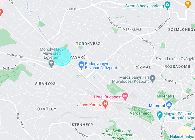
The fourth line uses the circle() method to add a circle to the plot.

The circle() method takes the latitude and longitude coordinates of the center of the circle as its first two arguments, followed by the radius of the circle in meters.

The face_alpha parameter specifies the transparency of the circle fill, while the ec and fc parameters specify the color of the circle edge and fill, respectively.

Polyline (plot)

A polyline is a line composed of one or more sections. If we want to display such a line on our map, we use the plot method. In addition to the usual lats [float], lons [float] parameters, you can specify the following optional parameters:

color/c/edge_color/ec str : Color of the polyline. Can be hex (“#00FFFF”), named (‘cyan’), or matplotlib-like (‘c’). Defaults to black.
alpha/edge_alpha/ea float: Opacity of the polyline, ranging from 0 to 1. Defaults to 1.0.
edge_width/ew int: Width of the polyline, in pixels. Defaults to 1.
precision int: Number of digits after the decimal to round to for lat/lng values. Defaults to 6.

import gmplot
apikey = ' ' # (your API key here)
gmap = gmplot.GoogleMapPlotter(47.519350864380385, 19.010462124312387, zoom = 14, apikey=apikey)
f = zip(*[(47.513285942712805, 18.994089961008104),
          (47.51453956566773, 18.991150259891935),
          (47.51573518971617, 18.992276787691928),
          (47.51453956566773, 18.991150259891935),
          (47.51417000363217, 18.992040753295736),
          (47.515372882275294, 18.99316728109573)])
gmap.plot(*f, edge_width = 7, color = 'limegreen')
gmap.draw('poly.html')

Result:

f = zip(*[(47.513285942712805, 18.994089961008104), (47.51453956566773, 18.991150259891935), (47.51573518971617, 18.992276787691928), (47.51453956566773, 18.991150259891935), (47.51417000363217, 18.992040753295736), (47.515372882275294, 18.99316728109573)])

This line creates a list of latitude-longitude pairs that define the vertices of a polygon. The zip(*[...]) function is used to transpose the list so that each pair of latitude-longitude values becomes a separate tuple.

gmap.plot(*f, edge_width = 7, color = 'limegreen')

This line plots the polygon on the Google Map. The plot() function takes the *f argument, which is unpacked as separate arguments, representing the latitude and longitude values of the polygon vertices. The edge_width parameter sets the width of the polygon edges in pixels and the color parameter sets the color of the edges.

Create heatmap (heatmap)

Plot a heatmap.

Parameters:

Latitudes [float],
Longitudes [float]

Optional Parameters:

radius [int]: Radius of influence for each data point, in pixels. Defaults to 10.
gradient [(int, int, int, float)]: Color gradient of the heatmap as a list of RGBA colors. The color order defines the gradient moving towards the center of a point.
opacity [float]: Opacity of the heatmap, ranging from 0 to 1. Defaults to 0.6.
max_intensity [int]: Maximum intensity of the heatmap. Defaults to 1.
dissipating [bool]: True to dissipate the heatmap on zooming, False to disable dissipation.
precision [int]: Number of digits after the decimal to round to for lat/lng values. Defaults to 6.
weights [float]: List of weights corresponding to each data point. Each point has a weight of 1 by default. Specifying a weight of N is equivalent to plotting the same point N times.

import gmplot
apikey = ' ' # (your API key here)
gmap = gmplot.GoogleMapPlotter(47.519350864380385, 19.010462124312387, zoom = 14, apikey=apikey)
letters = zip(*[
    (47.51471253011692, 18.990678878050492),
    (47.51941514547201, 18.993554206158933),
    (47.52134244386804, 18.998060317311538),
    (47.52337110249922, 19.002008528961046),
    (47.52344355313603, 19.009969325319076),
    (47.52466070898612, 19.013488383565445),
    (47.526645771633746, 19.02031192332838)])

gmap.heatmap(
    *letters,
    radius=55,
    weights=[0.1, 0.2, 0.5, 0.6, 1.8, 2.10, 1.12],
    gradient=[(89, 185, 90, 0), (54, 154, 211, 0.5), (254, 179, 19, 0.79), (227, 212, 45, 1)],
    opacity = 0.7
)
gmap.draw('heatmap.html')

Result:

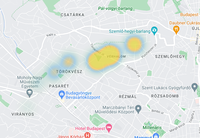
First, a list of tuples called letters is created. Each tuple contains two values representing latitude and longitude coordinates of a point on the map.

Then, an instance of the GoogleMapPlotter class is created with a specified center point, zoom level, and an API key.

Next, the heatmap method of the GoogleMapPlotter object is called, passing in the letters list as positional arguments, along with other parameters.

The radius parameter determines the radius of each data point’s influence on the heatmap, while the weights parameter determines the intensity of each data point’s contribution to the heatmap.

The gradient parameter is a list of tuples representing the color gradient of the heatmap, with each tuple containing four values representing red, green, blue, and alpha values.

Finally, the opacity parameter determines the transparency of the heatmap.

Picture above the map (ground_overlay)

Overlay an image from a given URL onto the map.

Parameters:

url [str]: URL of image to overlay.
bounds [dict]: Image bounds, as a dict of the form {'north':, 'south':, 'east':, 'west':}.

Optional Parameters:

opacity [float]: Opacity of the overlay, ranging from 0 to 1. Defaults to 1.0.

import gmplot
apikey = ' ' # (your API key here)
gmap = gmplot.GoogleMapPlotter(47.519350864380385, 19.010462124312387, zoom = 14, apikey=apikey)
url = 'https://finxter.com/wp-content/uploads/2022/01/image-2.png'
bounds = {'north': 47.53012124664374, 'south': 47.50860174660818, 'east': 19.0247910821219, 'west': 18.985823949220986}
gmap.ground_overlay(url, bounds, opacity=0.3)
gmap.draw('overlay.html')

Result:

The variable url contains the URL of an image that will be used as the ground overlay. The bounds dictionary defines the north, south, east, and west coordinates of the image on the map.

Finally, the ground_overlay method is called on the GoogleMapPlotter object, passing the URL and bounds variables as arguments. The opacity parameter is set to 0.3 to make the overlay partially transparent. The resulting map is saved to a file called overlay.html using the draw method.

Plot a Polygon

Parameters:

lats [float]: Latitudes.
lngs [float]: Longitudes.

Optional Parameters:

color/c/edge_color/ec str: Color of the polygon’s edge. Can be hex (“#00FFFF”), named (“cyan”), or matplotlib-like (“c”). Defaults to black.
alpha/edge_alpha/ea float: Opacity of the polygon’s edge, ranging from 0 to 1. Defaults to 1.0.
edge_width/ew int: Width of the polygon’s edge, in pixels. Defaults to 1.
alpha/face_alpha/fa float: Opacity of the polygon’s face, ranging from 0 to 1. Defaults to 0.3.
color/c/face_color/fc str: Color of the polygon’s face. Can be hex (“#00FFFF”), named (“cyan”), or matplotlib-like (“c”). Defaults to black.
precision int: Number of digits after the decimal to round to for lat/lng values. Defaults to 6.

import gmplot
apikey = ' ' # (your API key here)
gmap = gmplot.GoogleMapPlotter(47.519350864380385, 19.010462124312387, zoom = 14, apikey=apikey)
finxter_in_Budapest = zip(*[
        (47.53012124664374, 18.985823949220986),
        (47.53012124664374, 19.0247910821219),
        (47.50860174660818, 19.0247910821219),
        (47.50860174660818, 18.985823949220986),
        (47.53012124664374, 18.985823949220986)])

gmap.polygon(*finxter_in_Budapest, face_color='grey', face_alpha = 0.15, edge_color='cornflowerblue', edge_width=3)
gmap.draw('poligon.html')

Result:

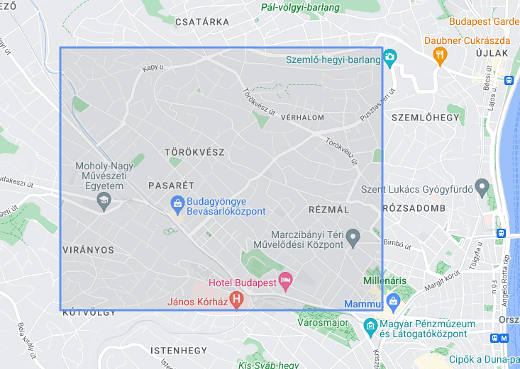
Defines a set of coordinates for a polygon named finxter_in_Budapest.

Calls the gmap.polygon() method with the *finxter_in_Budapest argument to draw the polygon on the map. The face_color, face_alpha, edge_color, and edge_width parameters define the appearance of the polygon.

Saves the map as an HTML file named 'poligon.html' using the gmap.draw() method.

Display grid (grid)

The parameters are used to specify the grid start and end points and the width and length of the grid.

(lat_start, lat_end, lat_increment, lng_start, lng_end, lng_increment)

import gmplot
apikey = ' ' # (your API key here)
gmap = gmplot.GoogleMapPlotter(47.519350864380385, 19.010462124312387, zoom = 14, apikey=apikey)
gmap.grid(47.50, 47.53, 0.0025, 19.0, 19.05, 0.0025)
gmap.draw('grid.html')

Result:

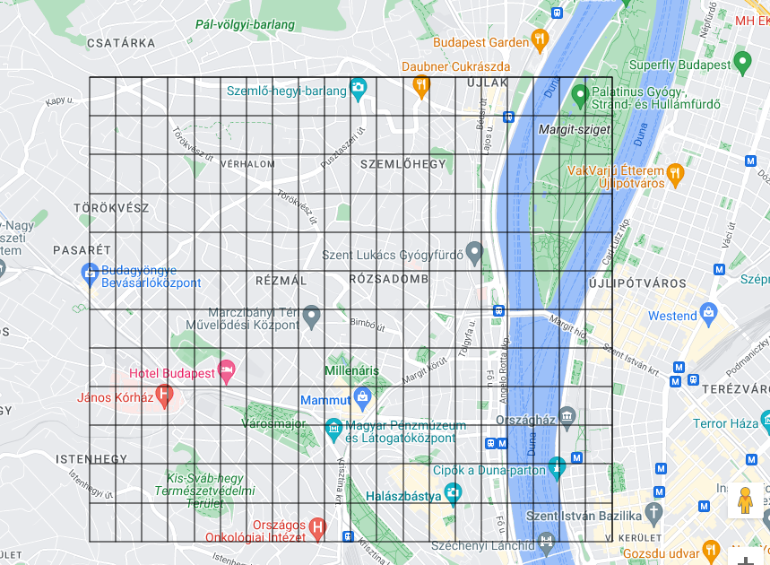
This code generates a Google Map centered at latitude 47.519350864380385 and longitude 19.010462124312387, with a zoom level of 14. It then adds a grid to the map with vertical lines spaced 0.0025 degrees apart between longitude 19.0 and 19.05, and horizontal lines spaced 0.0025 degrees apart between latitude 47.50 and 47.53. Finally, it saves the resulting map with the grid to an HTML file named "grid.html".

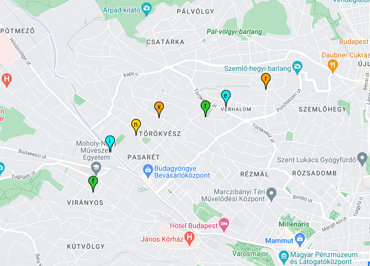
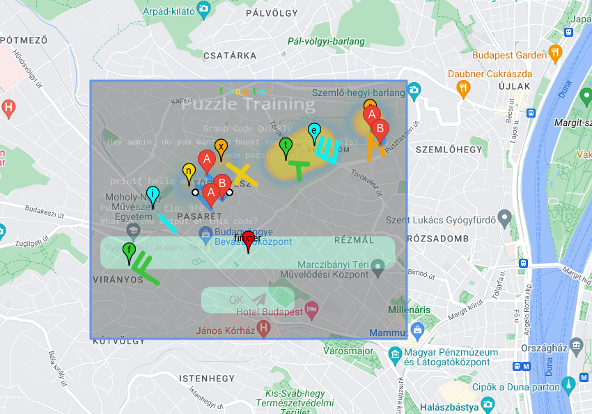
Let’s put it together and see where I found “finxter”!

Import module, create gmap instance

import gmplot
#apikey =  # (your API key here)
bounds = {'north': 47.623, 'south': 47.323, 'east': 19.208, 'west': 18.808}
gmap = gmplot.GoogleMapPlotter(47.519350864380385, 19.010462124312387, zoom = 13, fit_bounds=bounds, apikey=apikey)

Define letter direction routes

gmap.directions(
   (47.525977181062025, 19.02052238472371),
   (47.524798091352515, 19.021546988570606))
gmap.directions(
   (47.5194613766804, 19.000656008676216),
   (47.520243896650946, 19.00204002854648),
   waypoints = [(47.520888742275, 18.99871408933636)])

gmap.directions(
   (47.52226897515179, 19.00018393988221),
   (47.520243896650946, 19.00204002854648),
   waypoints = [(47.52088149688948, 19.002871513347902)])

Define letters routes

r = zip(*[
   (47.52356554300279, 19.02012541778466),
   (47.5259726531124, 19.020546524602626),
   (47.52484065497139, 19.020254163818944),
   (47.52481167549813, 19.021541624161788),
   (47.52479718575549, 19.021541624161788),
   (47.52398575378016, 19.021906404592265)])

e = zip(*[(47.52529997270366, 19.014375612740643),
         (47.52403211687861, 19.013828442094937),
         (47.52369884683277, 19.01479403735207),
         (47.52514058679826, 19.01530902148921),
         (47.52369884683277, 19.01479403735207),
         (47.52335832959914, 19.015786454699683),
         (47.524981200408554, 19.016301438836823)])

t = zip(*[(47.52326414357012, 19.01047031640738),
         (47.52316633484429, 19.012573168300694),
         (47.52319169267961, 19.011403725155944),
         (47.521873068989784, 19.01161830187975)])

x = zip(*[(47.52149735340168, 19.006154537181025),
         (47.52312028178215, 19.002850055634386),
         (47.522424747195465, 19.004411101300082),
         (47.52301522767022, 19.00516211983341),
         (47.522424747195465, 19.004411101300082),
         (47.52161690117839, 19.003729820201993)])

i = zip(*[(47.51762820549394, 18.996203541721567),
         (47.51873681072719, 18.994594216293006)])

f = zip(*[(47.513285942712805, 18.994089961008104),
         (47.51453956566773, 18.991150259891935),
         (47.51573518971617, 18.992276787691928),
         (47.51453956566773, 18.991150259891935)])

Plot the letters

gmap.plot(*r, edge_width = 7, color = 'orange')

gmap.plot(*e, edge_width = 7, color = 'c')

gmap.plot(*t, edge_width = 7, color = 'limegreen')

gmap.plot(*x, edge_width = 7, color = 'gold')

gmap.plot(*i, edge_width = 7, color = 'cyan')

gmap.plot(*f, edge_width = 7, color = 'limegreen')
gmap.circle(47.51894874729591, 18.99426698678921, 10, face_alpha = 1, ec = 'cyan', fc='cyan')

Create text on map:

finxter_text = ['f', 'i', 'n', 'x', 't', 'e', 'r']
colors = ['limegreen', 'cyan', 'gold','orange', 'limegreen', 'cyan', 'orange']
j = 0
lat = 47.529266431577625
lng = 19.00200303401821
for i in finxter_text:
   gmap.text(lat, lng, i, color = colors[j], size = 10)
   j += 1
   lng += 0.001

Drop a marker with finxter link, enable marker dropping:

gmap.marker(47.515703432784726, 19.005350430919034, label = 'finxter', info_window = "<a href='https://finxter.com/'>The finxter academy</a>")

gmap.enable_marker_dropping(color = 'black')

Define and plot scatter points for letters:

letters = zip(*[
   (47.51471253011692, 18.990678878050492),
   (47.51941514547201, 18.993554206158933),
   (47.52134244386804, 18.998060317311538),
   (47.52337110249922, 19.002008528961046),
   (47.52344355313603, 19.009969325319076),
   (47.52466070898612, 19.013488383565445),
   (47.526645771633746, 19.02031192332838)])

gmap.scatter(*letters,
   color=['limegreen', 'cyan','gold','orange', 'limegreen', 'cyan', 'orange'],
   s=60,
   ew=1,
   title=['f', 'i', 'n', 'x', 't', 'e', 'r'],
   label=['f', 'i', 'n', 'x', 't', 'e', 'r']
)

Create heatmap:

letters = zip(*[
   (47.51471253011692, 18.990678878050492),
   (47.51941514547201, 18.993554206158933),
   (47.52134244386804, 18.998060317311538),
   (47.52337110249922, 19.002008528961046),
   (47.52344355313603, 19.009969325319076),
   (47.52466070898612, 19.013488383565445),
   (47.526645771633746, 19.02031192332838)])

gmap.heatmap(
   *letters,
   radius=55,
   weights=[0.1, 0.2, 0.5, 0.6, 1.8, 2.10, 1.12],
   gradient=[(89, 185, 90, 0), (54, 154, 211, 0.5), (254, 179, 19, 0.79), (227, 212, 45, 1)],
   opacity = 0.7
)

Overlay image from URL:

url = 'https://finxter.com/wp-content/uploads/2022/01/image-2.png'
bounds = {'north': 47.53012124664374, 'south': 47.50860174660818, 'east': 19.0247910821219, 'west': 18.985823949220986}
gmap.ground_overlay(url, bounds, opacity=0.3)

Draw polygon:

finxter_in_Budapest = zip(*[
   (47.53012124664374, 18.985823949220986),
   (47.53012124664374, 19.0247910821219),
   (47.50860174660818, 19.0247910821219),
   (47.50860174660818, 18.985823949220986),
   (47.53012124664374, 18.985823949220986)])

gmap.polygon(*finxter_in_Budapest, face_color='grey', face_alpha = 0.15, edge_color='cornflowerblue', edge_width=3)

Draw map to file:

gmap.draw('finxter_in_budapest.html')

Output:

Conclusion

Congratulations, now you’ve learned how to draw almost anything on Google Maps with a few lines of code. While gmplot is a powerful library, it has some limitations (e.g., I can’t figure out how to change the color of the path), so maybe other modules like geopandas are a good place to learn more.

A Few Final Words on gmplot

gmplot is a Python library that allows the user to plot data on Google Maps. It provides a simple interface to create various types of maps, including scatterplots, heatmaps, ground overlays, and polygons.

With gmplot, the user can add markers, lines, and shapes to the map, customize colors, labels, and other properties, and export the map to a static HTML file.

The library uses the Google Maps API and requires an API key to be able to use it. gmplot is a useful tool for visualizing geospatial data and creating interactive maps for data exploration and analysis.

April 01, 2023 at 04:30PM
Click here for more details...

=============================
The original post is available in Be on the Right Side of Change by Gábor Madarász
this post has been published as it is through automation. Automation script brings all the top bloggers post under a single umbrella.
The purpose of this blog, Follow the top Salesforce bloggers and collect all blogs in a single place through automation.
============================

Gábor Madarász Python

Python Reader

I Created a Python Program to Find Strings on Google Maps (e.g,. “Finxter” in Budapest) : Gábor Madarász

GoogleMapPlotter

Find a location by name (from_geocode)

Coordinates of a location (geocode)

Text on your map (text)

Drop marker (marker)

gmap.enable_marker_dropping(color=’black’)

Route planning (directions)

Display many points (scatter)

Draw circle (circle)

Polyline (plot)

Create heatmap (heatmap)

Picture above the map (ground_overlay)

Plot a Polygon

Display grid (grid)

Let’s put it together and see where I found “finxter”!

Conclusion

A Few Final Words on gmplot

Post a Comment