Understanding Tasks in Diffusers: Part 3 : Aritra Roy Gosthipaty and Ritwik Raha
by: Aritra Roy Gosthipaty and Ritwik Raha
blow post content copied from PyImageSearch
click here to view original post
Table of Contents
- Understanding Tasks in Diffusers: Part 3
- Introduction
- Why Not Image-to-Image?
- ControlNet Models
- Configuring Your Development Environment
- Setup and Imports
- Utility Functions
- Canny ControlNet
- Pose ControlNet
- Load Dancer Image
- Detect Pose
- Load ControlNet Model
- Load and Configure Pipeline
- Image Generation
- Cleaning Up
- Depth ControlNet
- Load Depth Estimation Model
- Load Image and Extract Depth
- Load ControlNet Model
- Load and Configure Pipeline (Skipping Safety Check)
- Image Generation
- Cleaning Up
- Segmentation Map ControlNet
- Summary
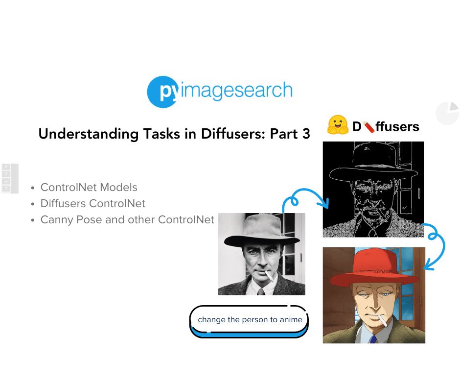
Understanding Tasks in Diffusers: Part 3
In this tutorial, you will learn how to control specific aspects of text-to-image with spatial information.
This lesson is the last of a 3-part series on Understanding Tasks in Diffusers:
- Understanding Tasks in Diffusers: Part 1
- Understanding Tasks in Diffusers: Part 2
- Understanding Tasks in Diffusers: Part 3 (this tutorial)
To learn how to use ControlNet in Diffusers, just keep reading.
Understanding Tasks in Diffusers: Part 3
Introduction
This is the last of a 3-part series on Understanding Tasks in Diffusers. Today, we are looking at a special kind of task known as ControlNet.
Imagine being able to prompt your image generations with the spatial information of the images along with texts for better guidance.
This unlocks the ability to use edges, depths, and other spatial cues that mimic the original picture.
Why Not Image-to-Image?
➤ The answer is Control. Yes, that gives the architecture its name.
➤ ControlNet improves text-to-image generation by adding user control. Traditional models create impressive visuals but need more precision. ControlNet allows extra information, like sketches or depth data, to be included alongside text descriptions. This guides the model to create images that better match the user’s idea. Imagine creating a basic outline and letting the AI turn it into a complete image. This opens possibilities in art, design, and simulations, giving users more control over the final image
A Note of Acknowledgement: This tutorial was inspired in part by the official documentation from Hugging Face Diffusers.
ControlNet Models
Zhang, Rao, and Agrawala (2023) introduced the ControlNet method in their paper, Adding Conditional Control to Text-to-Image Diffusion Models.
It introduces a framework for supporting various spatial contexts, which can serve as additional conditionings to Diffusion models such as Stable Diffusion.
- The entire code base is open-sourced here.
- Over the past year, the community has submitted an insane number of applications for custom ControlNet models. Here is a non-exhaustive list of some of the Colab notebooks.
A sample from the paper is shown in Figure 1.
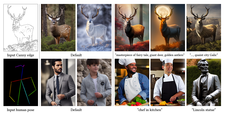
Any conditioning requires training a new copy of ControlNet weights.
The original paper proposed 8 different conditioning models that are all supported in Diffusers!
So, considering all the possible applications and outcomes of ControlNet, let’s look at how we can use various ControlNet Models to generate images as we want them.
Although, as mentioned before, the official paper and corresponding repository have 8 different ControlNet models, in this tutorial, we will be looking at 4 of the most popular and well-used models:
- Canny ControlNet
- Pose ControlNet
- Depth ControlNet
- Segmentation Map ControlNet
Configuring Your Development Environment
To follow this guide, you need to have the diffusers library installed on your system.
Luckily, diffusers is pip-installable:
$ pip install diffusers accelerate
If you need help configuring your development environment for OpenCV, we highly recommend that you read our pip install OpenCV guide — it will have you up and running in minutes.
Need Help Configuring Your Development Environment?
All that said, are you:
- Short on time?
- Learning on your employer’s administratively locked system?
- Wanting to skip the hassle of fighting with the command line, package managers, and virtual environments?
- Ready to run the code immediately on your Windows, macOS, or Linux system?
Then join PyImageSearch University today!
Gain access to Jupyter Notebooks for this tutorial and other PyImageSearch guides pre-configured to run on Google Colab’s ecosystem right in your web browser! No installation required.
And best of all, these Jupyter Notebooks will run on Windows, macOS, and Linux!
Setup and Imports
Installation
!pip install -q opencv-contrib-python
!pip install -q controlnet_aux
We install libraries for diffusion models (diffusers, transformers), computer vision (opencv-contrib-python), and a custom library (controlnet_aux).
Imports
import torch
import cv2
import numpy as np
from PIL import Image
from transformers import pipeline, AutoImageProcessor, UperNetForSemanticSegmentation
from diffusers import UniPCMultistepScheduler
from diffusers import StableDiffusionControlNetPipeline
from diffusers.utils import load_image
from diffusers import StableDiffusionControlNetPipeline, ControlNetModel
from controlnet_aux import OpenposeDetector, HEDdetector
We import functionalities from these libraries to work with images (torch, cv2, numpy, PIL), potentially use pre-trained models (transformers), and leverage diffusion models with control (diffusers, controlnet_aux).
Utility Functions
These functions provide helpful tools for processing images:
def create_canny_image(image):
    image = np.array(image)
    low_threshold = 100
    high_threshold = 200
    image = cv2.Canny(image, low_threshold, high_threshold)
    image = image[:, :, None]
    image = np.concatenate([image, image, image], axis=2)
    canny_image = Image.fromarray(image)
    return canny_image
create_canny_image(image): This function takes an image as input and returns a new image highlighting its edges. Here’s a breakdown of what it does:
- We convert the image to a NumPy array for easier manipulation with OpenCV.
- We define two thresholds,
low_thresholdandhigh_threshold, to control the sensitivity of edge detection. Lower values detect more edges, while higher values detect only strong edges. - We use OpenCV’s
cv2.Cannyfunction to apply the Canny edge filter with the defined thresholds, effectively identifying edges in the image. - Since OpenCV’s
Cannyreturns a single-channel grayscale image, we convert it to a three-channel RGB image (required for thePIL.Imagelibrary) by duplicating the channel. - We create a new
PIL.Imageobject from the processed NumPy array, resulting in an image with highlighted edges. - Finally, the function returns this new edge-enhanced image.
def image_grid(imgs, rows, cols):
    assert len(imgs) == rows * cols

    w, h = imgs[0].size
    grid = Image.new("RGB", size=(cols * w, rows * h))
    grid_w, grid_h = grid.size

    for i, img in enumerate(imgs):
        grid.paste(img, box=(i % cols * w, i // cols * h))
    return grid
image_grid(imgs, rows, cols): This function takes a list of images (imgs), the desired number of rows (rows), and columns (cols) and arranges them into a single grid image. Here’s what it does:
- We first check if the total number of images (
len(imgs)) matches the product of rows and columns (ensuring we have enough images to fill the grid). - We then retrieve the width (
w) and height (h) of the first image as a reference for the grid size. - We create a new empty
PIL.Imageobject in RGB mode with dimensions calculated by multiplying the number of columns by the image width and rows by the image height, effectively creating a canvas for the grid. - We iterate through each image in the list and paste it onto the grid image at the corresponding position determined by its index (
i). The modulo (%) operation calculates the column position, and integer division (//) calculates the row position within the grid. - Finally, the function returns the combined grid image containing all the input images arranged as specified.
def delete_pipeline(pipeline):
    pipeline.to("cpu")
    del pipeline
    torch.cuda.empty_cache()
delete_pipeline(pipeline): This function takes a loaded Stable Diffusion pipeline (pipeline) as input and properly removes it from memory. Here’s what it does:
- First, we move the pipeline to the CPU (if it was previously on the GPU) to avoid memory leaks.
- Then, we use the
delstatement to explicitly delete the pipeline object, freeing up the memory it occupies. - Lastly, we call
torch.cuda.empty_cache()to ensure any remaining cached GPU memory associated with the pipeline is cleared as well. This helps maintain efficient memory usage, especially when dealing with multiple pipelines.
Canny ControlNet
This code snippet demonstrates how to leverage a pre-trained diffusion model along with a control network to generate images based on a prompt while incorporating edge information from another image. Let’s break down the steps and visualize the image in Figure 2:
prompt = "Oppenheimer as an anime character, high definition best quality, extremely detailed"
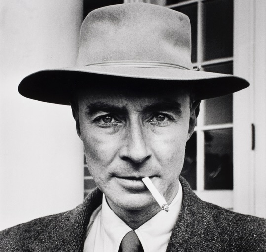
image = load_image(
"https://huggingface.co/datasets/ritwikraha/random-storage/resolve/main/oppenheimer.png"
)
image
Setting Up
- We define a prompt describing the desired image (“Oppenheimer as an anime character, high definition best quality, extremely detailed”).
- We load an image of Oppenheimer (“https://huggingface.co/datasets/ritwikraha/random-storage/resolve/main/oppenheimer.png“) using the
load_imagefunction. - Using the
create_canny_imagefunction, we create a new image highlighting the edges of the loaded image. This edge information will guide the diffusion process. Let’s look at the edge map in Figure 3.
canny_image = create_canny_image(image)
canny_image
controlnet = ControlNetModel.from_pretrained("lllyasviel/sd-controlnet-canny", torch_dtype=torch.float16)
pipe = StableDiffusionControlNetPipeline.from_pretrained(
    "runwayml/stable-diffusion-v1-5", controlnet=controlnet, torch_dtype=torch.float16
)

pipe.scheduler = UniPCMultistepScheduler.from_config(pipe.scheduler.config)
pipe.enable_model_cpu_offload()
pipe.enable_xformers_memory_efficient_attention()
Loading the Model
- We load a pre-trained
ControlNetModelcalled “sd-controlnet-canny” from the Hugging Face Hub. This model is specifically designed to work with Canny edge images for control. - We load a pre-trained Stable Diffusion pipeline (“runwayml/stable-diffusion-v1-5”) and integrate the loaded
controlnetmodel into the pipeline. We also specifytorch.float16for using a lower-precision data type to save memory, if possible, on your hardware.
Optimizing the Pipeline
- We configure the pipeline’s scheduler using
UniPCMultistepScheduler.from_configfor potentially better performance during image generation. - We enable CPU offloading (
enable_model_cpu_offload) to move the model to the CPU if a GPU is available, potentially improving memory usage on systems with limited GPU memory. - We enable memory-efficient attention (
enable_xformers_memory_efficient_attention) to reduce memory consumption during image generation, especially for larger image sizes.
Image Generation
output = pipe(
    prompt,
    canny_image,
    negative_prompt="monochrome, low quality, lowres, bad anatomy, worst quality, low quality",
    num_inference_steps=20,
).images[0]

output
- We use the pipeline (
pipe) to generate an image based on the provided prompt (prompt). - We also include the created canny image (
canny_image) as an additional input to the pipeline. This injects the edge information to guide the diffusion process toward generating an image that aligns with the edges. - We provide a negative prompt (“monochrome, low quality, lowres, bad anatomy, worst quality, low quality”) to steer the generation away from unwanted qualities.
- We set the number of inference steps (
num_inference_steps) to20, which controls the detail and quality of the generated image (more steps typically lead to better results but take longer). - Finally, we run the pipeline, store the generated image in the
outputvariable, and display the image as shown in Figure 4.

Cleaning Up
delete_pipeline(pipe)
- After using the pipeline, we call the
delete_pipelinefunction to remove it from memory and free up resources properly. This is especially important when dealing with multiple pipelines.
Pose ControlNet
This code demonstrates using a pre-trained diffusion model with a control network that leverages human pose (from any image like in Figure 5) information for image generation. Let’s break it down step by step:
img_pose = load_image("https://huggingface.co/datasets/ritwikraha/random-storage/resolve/main/dancer.png")
img_pose
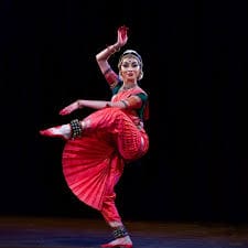
Load Dancer Image
- We load an image of a dancer (“https://huggingface.co/datasets/ritwikraha/random-storage/resolve/main/dancer.png“) using the
load_imagefunction.
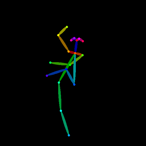
Detect Pose
model = OpenposeDetector.from_pretrained("lllyasviel/ControlNet")
pose = model(img_pose)
pose
- We load a pre-trained
OpenposeDetectormodel called “lllyasviel/ControlNet”. This model is designed to detect human poses from images. - We call the model (
model) on the loaded image (img_pose) to extract the human pose information. - The output (
pose) likely contains data representing the detected key points (e.g., shoulders, elbows, wrists) of the person in the image, as shown in Figure 6.
controlnet = ControlNetModel.from_pretrained(
    "fusing/stable-diffusion-v1-5-controlnet-openpose", torch_dtype=torch.float16
)

model_id = "runwayml/stable-diffusion-v1-5"
pipe = StableDiffusionControlNetPipeline.from_pretrained(
    model_id,
    controlnet=controlnet,
    torch_dtype=torch.float16,
)
pipe.scheduler = UniPCMultistepScheduler.from_config(pipe.scheduler.config)
pipe.enable_model_cpu_offload()
pipe.enable_xformers_memory_efficient_attention()
Load ControlNet Model
- We load a pre-trained
ControlNetModelcalledfusing/stable-diffusion-v1-5-controlnet-openposespecifically designed to work with OpenPose data for control. This model will use the extracted pose information to guide the image generation process.
Load and Configure Pipeline
- We define the Stable Diffusion model ID (“runwayml/stable-diffusion-v1-5”).
- We create a
StableDiffusionControlNetPipelineusing the loadedcontrolnetmodel and the specified model ID. We also specifytorch.float16to potentially save memory. - We configure the pipeline’s scheduler using
UniPCMultistepScheduler.from_configfor potentially better performance. - To potentially save memory, we enable CPU offloading (
enable_model_cpu_offload) and memory-efficient attention (enable_xformers_memory_efficient_attention).
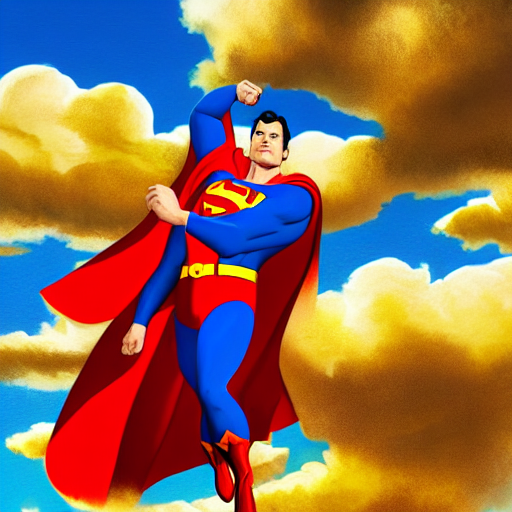
Image Generation
prompt = "illustration of superman flying to the sky, high definition best quality, extremely detailed"
output = pipe(
    prompt,
    pose,
    negative_prompt="monochrome, blurry, unclear face, missing body parts, extra digits, extra eyes, ugly, lowres, bad anatomy, worst quality, low quality",
    num_inference_steps=50,
).images[0]
output
- We define a prompt describing the desired image (“illustration of superman flying to the sky, high definition best quality, extremely detailed”).
- We use the pipeline (
pipe) to generate an image.
We provide the prompt (prompt) and the extracted pose information (pose) as inputs to the pipeline. The control network will use the pose information to influence the generation process, potentially aligning the generated Superman with a pose similar to that of the dancer in the loaded image.
- We include a negative prompt (“monochrome, blurry, unclear face, missing body parts, extra digits, extra eyes, ugly, lowres, bad anatomy, worst quality, low quality”) to steer the generation away from unwanted features.
We set the number of inference steps (num_inference_steps) to 50 for potentially higher-quality results (which may take longer).
- Finally, we run the pipeline and store the generated image in the
outputvariable. The final image is shown in Figure 7.
Cleaning Up
delete_pipeline(pipe)
After using the pipeline, we call the delete_pipeline function to properly remove it from memory and free up resources.
Depth ControlNet
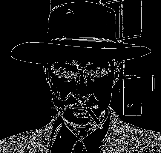
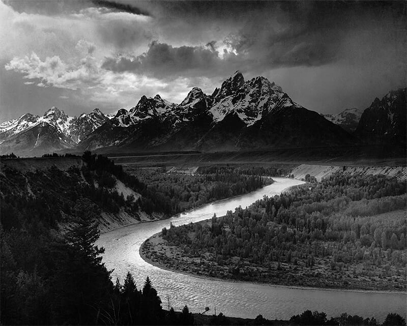
This code snippet demonstrates leveraging a pre-trained diffusion model with a control network that utilizes a depth map to guide image generation. We use a normal image (as shown in Figure 8) and use a depth-estimator model to generate its depth map. Here’s a breakdown:
depth_estimator = pipeline('depth-estimation')

image = load_image("https://huggingface.co/datasets/ritwikraha/random-storage/resolve/main/ansel.png")

image = depth_estimator(image)['depth']
image = np.array(image)
image = image[:, :, None]
image = np.concatenate([image, image, image], axis=2)
image = Image.fromarray(image)
Load Depth Estimation Model
We first load a pre-trained pipeline component (depth-estimation), likely using a model from the Hugging Face Hub. This component estimates depth information from an image.
Load Image and Extract Depth
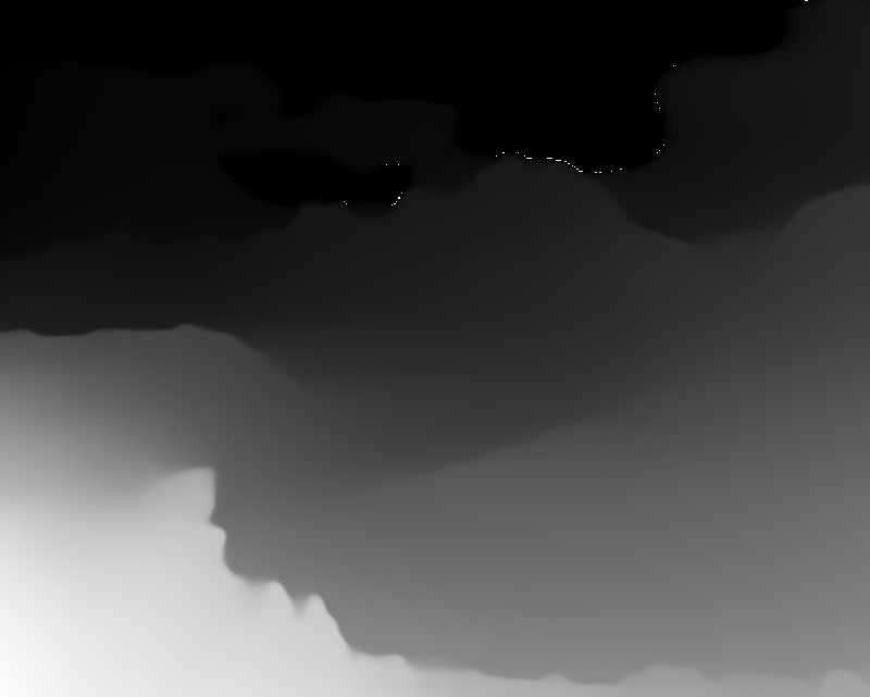
- We load an image of Ansel (“[https://huggingface.co/datasets/ritwikraha/random-storage/resolve/main/ansel.png](https://huggingface.co/datasets/ritwikraha/random-storage/resolve/main/ansel.png)”) using
load_image. - We use the loaded pipeline (
depth_estimator) on the image to extract the estimated depth information. The output (image) likely contains a single-channel grayscale image representing the predicted depth, where brighter values indicate closer objects, as shown in Figure 9. - We convert the depth image to a NumPy array for further processing.
- To make it compatible with the
PIL.Imagelibrary, we convert the single-channel depth image to a three-channel RGB image by duplicating the channel and then creating a newPIL.Imageobject from the processed array.
image
controlnet = ControlNetModel.from_pretrained(
    "lllyasviel/sd-controlnet-depth", torch_dtype=torch.float16
)

pipe = StableDiffusionControlNetPipeline.from_pretrained(
    "runwayml/stable-diffusion-v1-5", controlnet=controlnet, safety_checker=None, torch_dtype=torch.float16
)


pipe.scheduler = UniPCMultistepScheduler.from_config(pipe.scheduler.config)
pipe.enable_xformers_memory_efficient_attention()
pipe.enable_model_cpu_offload()
Load ControlNet Model
- We load a pre-trained
ControlNetModelcalled “lllyasviel/sd-controlnet-depth” specifically designed to work with depth information for control. This model will use the estimated depth to influence how the diffusion process generates the image.
Load and Configure Pipeline (Skipping Safety Check)
- We create a
StableDiffusionControlNetPipelineusing the loadedcontrolnetmodel and the specified Stable Diffusion model ID (“runwayml/stable-diffusion-v1-5”). We also specifytorch.float16for potential memory savings. - Important Note: We turn off the
safety_checkerby setting it toNone. This is likely for demonstration purposes only, and safety checks are usually recommended to prevent the generation of potentially harmful content. - We configure the pipeline’s scheduler using
UniPCMultistepScheduler.from_configfor potentially better performance. - To potentially save memory, we enable memory-efficient attention (
enable_xformers_memory_efficient_attention) and CPU offloading (enable_model_cpu_offload).
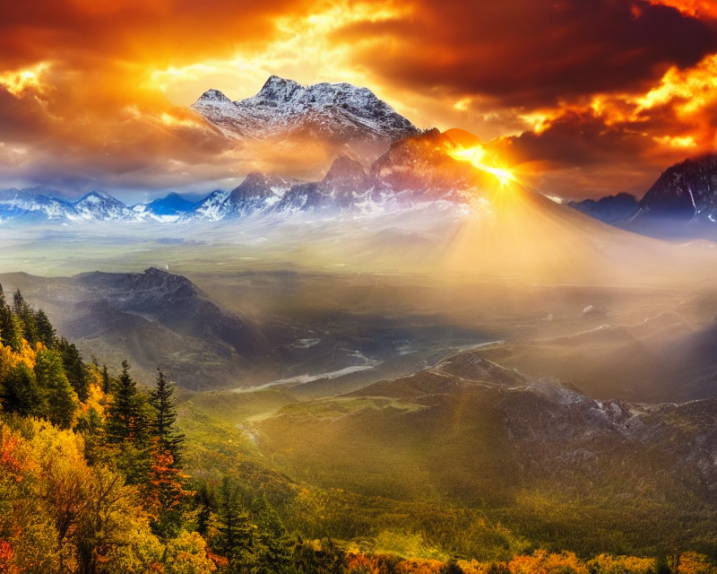
Image Generation
output = pipe("a looming mountain range, animated, high definition, high quality",
              image,
              negative_prompt ="monochrome, blurry, unclear face, missing body parts, extra digits, extra eyes, ugly, lowres, bad anatomy, worst quality, low quality",
              num_inference_steps=60).images[0]
output
- We define a prompt describing the desired image (“a looming mountain range, animated, high definition, high quality”).
- We use the pipeline (
pipe) to generate an image. - We provide the prompt (
prompt) and the extracted depth information (image) as inputs to the pipeline. The control network will use the depth information to potentially influence the generated image, emphasizing areas with predicted closer depth (potentially making the mountain range appear more prominent). - We include a negative prompt (“monochrome, blurry, unclear face, missing body parts, extra digits, extra eyes, ugly, lowres, bad anatomy, worst quality, low quality”) to steer the generation away from unwanted features.
- We set the number of inference steps (
num_inference_steps) to60for potentially higher-quality results (which may take longer). - Finally, we run the pipeline and store the generated image in the
outputvariable. The final image, as generated, is shown in Figure 10.
Cleaning Up
delete_pipeline(pipe)
- After using the pipeline, we call the
delete_pipelinefunction to remove it from memory and free up resources properly.
Important Note: Disabling the safety checker is not recommended for real-world applications. It’s crucial to ensure the responsible use of these models and avoid generating harmful content.
Segmentation Map ControlNet
This code snippet demonstrates leveraging a pre-trained diffusion model with a control network that utilizes segmentation information to guide image generation. In short, we take a normal image (as shown in Figure 11), generate a segmentation map from it, and then use that segmentation map as a guide for text-to-image generation. Here’s a breakdown of the steps:

Load the Palette
palette = np.asarray([
    [0, 0, 0],
    [120, 120, 120],
    [180, 120, 120],
    [6, 230, 230],
    [80, 50, 50],
    [4, 200, 3],
    [120, 120, 80],
    [...],
    [...],
    [92, 0, 255],
])
image_processor = AutoImageProcessor.from_pretrained("openmmlab/upernet-convnext-small")
image_segmentor = UperNetForSemanticSegmentation.from_pretrained("openmmlab/upernet-convnext-small")
Load Segmentation Model and Palette
- We define a color palette (
palette) containing a large number of colors mapped to different segment labels. This palette will be used later to colorize the segmentation output. - We load a pre-trained
AutoImageProcessorand aUperNetForSemanticSegmentationmodel from the OpenMMLab library. These models are likely trained for semantic segmentation, which aims to classify each pixel in an image into a specific category (e.g., sky, water, building).
Generate Segmentation Map
image = load_image("https://huggingface.co/datasets/ritwikraha/random-storage/resolve/main/sydney.png").convert('RGB')
pixel_values = image_processor(image, return_tensors="pt").pixel_values
with torch.no_grad():
  outputs = image_segmentor(pixel_values)

seg = image_processor.post_process_semantic_segmentation(outputs, target_sizes=[image.size[::-1]])[0]

color_seg = np.zeros((seg.shape[0], seg.shape[1], 3), dtype=np.uint8) # height, width, 3

for label, color in enumerate(palette):
    color_seg[seg == label, :] = color

color_seg = color_seg.astype(np.uint8)

image = Image.fromarray(color_seg)
image
Load and Segment Image
- We load an image of Sydney Opera House (“[https://huggingface.co/datasets/ritwikraha/random-storage/resolve/main/sydney.png](https://huggingface.co/datasets/ritwikraha/random-storage/resolve/main/sydney.png)”) and convert it to RGB format (required for the segmentation model).
- We use the loaded image processor (
image_processor) to prepare the image for the segmentation model by converting it to a format the model expects (tensors). - We turn off gradient calculation (
with torch.no_grad()) to improve efficiency, as we’re not backpropagating through the segmentation model in this case. - We use the segmentation model (
image_segmentor) to predict a segmentation mask for the image. This mask assigns a label to each pixel, potentially representing categories (e.g., sky, water, building, etc.).
Process and Colorize Segmentation
- We use the image processor’s post-processing function (
post_process_semantic_segmentation) to convert the model’s raw segmentation output into a more usable format. - We create a new empty image (
color_seg) with dimensions matching the segmentation mask and set the data type to unsigned 8-bit integers for efficient color representation. - We iterate through each unique label in the segmentation mask and its corresponding color from the defined palette (
palette). - For each pixel in the segmentation mask, we assign the corresponding color from the palette based on the predicted label, effectively creating a color-coded segmentation image where different colors represent different predicted categories.
- Finally, we convert the colorized segmentation image to an
Imageobject for further use. The final image is shown in Figure 12.

Loading the ControlNet Pipeline
controlnet = ControlNetModel.from_pretrained(
    "lllyasviel/sd-controlnet-seg", torch_dtype=torch.float16
)

pipe = StableDiffusionControlNetPipeline.from_pretrained(
    "runwayml/stable-diffusion-v1-5", controlnet=controlnet, safety_checker=None, torch_dtype=torch.float16
)

pipe.scheduler = UniPCMultistepScheduler.from_config(pipe.scheduler.config)
pipe.enable_xformers_memory_efficient_attention()
pipe.enable_model_cpu_offload()
Load ControlNet and Pipeline (Skipping Safety Check)
- We load a pre-trained
ControlNetModelcalled “lllyasviel/sd-controlnet-seg” specifically designed to work with segmentation information for control. This model will use the segmentation information to influence how the diffusion process generates the image. - We create a
StableDiffusionControlNetPipelineusing the loadedcontrolnetmodel and the specified Stable Diffusion model ID (“runwayml/stable-diffusion-v1-5”). We also specifytorch.float16for potential memory savings. - Important Note: We turn off the
safety_checkerby setting it toNone. This is likely for demonstration purposes only, and safety checks are usually recommended to prevent the generation of potentially harmful content. - We configure the pipeline’s scheduler using
UniPCMultistepScheduler.from_configfor potentially better performance. - To potentially save memory, we enable memory-efficient attention (
enable_xformers_memory_efficient_attention) and CPU offloading (enable_model_cpu_offload).
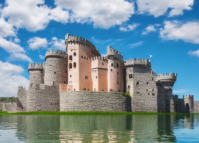
Image Generation
output = pipe("a magnificient castle on a lake with clear sky above",
              image,
              num_inference_steps=50).images[0]
output
- We define a prompt describing the desired image (“a magnificent castle on a lake with clear sky above”).
- We use the pipeline (
pipe) to generate an image. - We provide the prompt (
prompt) and the colorized segmentation image (image) as inputs to the pipeline. The control network will use the segmentation information to influence the generated image potentially, aligning certain aspects with the predicted categories in the segmentation (e.g., placing the castle on a region predicted as water in the segmentation). - We set the number of inference steps (
num_inference_steps) to50for potentially higher-quality results (which may take longer). - Finally, we run the pipeline and store the generated image in the
outputvariable. The final image is shown in Figure 13.
Cleaning Up
delete_pipeline(pipe)
- After using the pipeline, we call the
delete_pipelinefunction to remove it from memory and free up resources properly.
Important Note: Disabling the safety checker is not recommended for real-world applications. It’s crucial to ensure the responsible use of these models and avoid generating harmful content.
What's next? We recommend PyImageSearch University.
84 total classes • 114+ hours of on-demand code walkthrough videos • Last updated: February 2024
★★★★★ 4.84 (128 Ratings) • 16,000+ Students Enrolled
I strongly believe that if you had the right teacher you could master computer vision and deep learning.
Do you think learning computer vision and deep learning has to be time-consuming, overwhelming, and complicated? Or has to involve complex mathematics and equations? Or requires a degree in computer science?
That’s not the case.
All you need to master computer vision and deep learning is for someone to explain things to you in simple, intuitive terms. And that’s exactly what I do. My mission is to change education and how complex Artificial Intelligence topics are taught.
If you're serious about learning computer vision, your next stop should be PyImageSearch University, the most comprehensive computer vision, deep learning, and OpenCV course online today. Here you’ll learn how to successfully and confidently apply computer vision to your work, research, and projects. Join me in computer vision mastery.
Inside PyImageSearch University you'll find:
- ✓ 84 courses on essential computer vision, deep learning, and OpenCV topics
- ✓ 84 Certificates of Completion
- ✓ 114+ hours of on-demand video
- ✓ Brand new courses released regularly, ensuring you can keep up with state-of-the-art techniques
- ✓ Pre-configured Jupyter Notebooks in Google Colab
- ✓ Run all code examples in your web browser — works on Windows, macOS, and Linux (no dev environment configuration required!)
- ✓ Access to centralized code repos for all 536+ tutorials on PyImageSearch
- ✓ Easy one-click downloads for code, datasets, pre-trained models, etc.
- ✓ Access on mobile, laptop, desktop, etc.
Summary
As we close this chapter, let us rewind to understand what was the primary objectives:
- ControlNet Models help us to perfectly guide the denoising process both with a text prompt and with spatial signals.
- The original paper released multiple ControlNet models, of which 4 have been showcased here.
- Additionally, you can also fuse two ControlNet Models by adding your ControlNet models to a list and the input images to a list.
- ControlNet models also allow the workflow to be paired with other models like a pose estimation model or a segmentation model. This opens up avenues for many applications.
Let us try to understand a few of them.
Applications of ControlNet in the Industry
Personalized Media and Advertising
- Application: Customized content generation for marketing and advertising.
- Technical Details: ControlNet can be used to adapt promotional materials to reflect diverse consumer profiles or scenarios, effectively personalizing advertising imagery to suit different demographics, locations, and individual preferences.
- Example: Using ControlNet to generate custom images of products in settings that align with the target audience’s lifestyle, such as changing the background or contextual elements of an image to fit urban or rural settings.
Interactive Entertainment and Gaming
- Application: Dynamic environment generation based on player interaction and choices.
- Technical Details: In video games or VR environments, ControlNet can dynamically modify visuals in real-time to adapt to player inputs or narrative changes, enhancing the immersive experience.
- Example: Adjusting the appearance and style of game environments and characters based on player decisions or environmental factors enhances the game’s adaptability and engagement.
Automotive Industry
- Application: Enhanced simulation for autonomous vehicle testing.
- Technical Details: ControlNet can generate varied traffic scenarios under different conditions during the simulation phase of autonomous vehicle development, improving the robustness of the vehicles’ perception systems.
- Example: Simulating different weather conditions, traffic densities, and pedestrian scenarios to train autonomous driving systems, helping them adapt to real-world variables.
Medical Imaging
- Application: Customizable medical training tools and enhanced diagnostic visuals.
- Technical Details: For medical training and diagnostics, ControlNet can be employed to generate anatomically accurate images under various simulated medical conditions, aiding in education and diagnostic processes.
- Example: Creating detailed and condition-specific images (e.g., varying stages of a disease or responses to treatments), which can be used for training medical professionals or for planning surgeries.
Architectural Visualization and Urban Planning
- Application: Adaptive visualization of architectural designs and urban layouts.
- Technical Details: Architects and planners can use ControlNet to visualize architectural projects or urban designs under different contextual scenarios (e.g., varying light conditions, seasons, or surrounding developments).
- Example: Generating images of how a building would look at different times of the day or year or simulating the visual impact of a new building on the existing urban landscape.
Fashion and Design
- Application: Tailored design visualizations reflecting contextual customer preferences.
- Technical Details: In fashion, ControlNet can be used to create images of apparel or products in different styles, settings, or models of varying body types, reflecting a more diverse range of consumer profiles.
- Example: Showcasing clothing items in different urban or natural settings on models of various body types and ethnic backgrounds to cater to a global market.
These applications leverage the unique ability of ControlNet to incorporate specific, controlled variations into the generative process, enhancing both the flexibility and utility of diffusion models across a broad spectrum of industries.
What other applications can you think of? Let us know
@pyimagesearch
Citation Information
A. R. Gosthipaty and R. Raha. “Understanding Tasks in Diffusers: Part 3,” PyImageSearch, P. Chugh, A. R. Gosthipaty, S. Huot, K. Kidriavsteva, and R. Raha, eds., 2024, https://pyimg.co/ks4d0
@incollection{ARG-RR_2024_Understanding-Tasks-in-Diffusers-Part-3,
  author = {Aritra Roy Gosthipaty and Ritwik Raha},
  title = {Understanding Tasks in Diffusers: Part 3},
  booktitle = {PyImageSearch},
  editor = {Puneet Chugh and Susan Huot and Kseniia Kidriavsteva},
  year = {2024},
  url = {https://pyimg.co/ks4d0},
}

Join the PyImageSearch Newsletter and Grab My FREE 17-page Resource Guide PDF
Enter your email address below to join the PyImageSearch Newsletter and download my FREE 17-page Resource Guide PDF on Computer Vision, OpenCV, and Deep Learning.
The post Understanding Tasks in Diffusers: Part 3 appeared first on PyImageSearch.
May 27, 2024 at 06:30PM
Click here for more details...
=============================
The original post is available in PyImageSearch by Aritra Roy Gosthipaty and Ritwik Raha
this post has been published as it is through automation. Automation script brings all the top bloggers post under a single umbrella.
The purpose of this blog, Follow the top Salesforce bloggers and collect all blogs in a single place through automation.
============================


Post a Comment