A Deep Dive into Transformers with TensorFlow and Keras: Part 2 : Aritra Roy Gosthipaty and Ritwik Raha
by: Aritra Roy Gosthipaty and Ritwik Raha
blow post content copied from PyImageSearch
click here to view original post
Table of Contents
A Deep Dive into Transformers with TensorFlow and Keras: Part 2
In this tutorial, you will learn about the connecting parts of the Transformers architecture that hold together the encoder and decoder.
This lesson is the 2nd in a 3-part series on NLP 104:
- A Deep Dive into Transformers with TensorFlow and Keras: Part 1
- A Deep Dive into Transformers with TensorFlow and Keras: Part 2 (today’s tutorial)
- A Deep Dive into Transformers with TensorFlow and Keras: Part 3
To learn how the transformers architecture stitches together the multi-head attention layer with other components, just keep reading.
A Deep Dive into Transformers with TensorFlow and Keras: Part 2
A Brief Recap
In the previous tutorial, we studied the evolution of attention from its simplest form into Multi-Head Attention as we see today. In Video 1, we illustrate how the Input matrix is projected into the Query, Key, and Value Matrices.
Video 1: Projecting the Input matrix into the Query, Key, and Value matrices.
Here the Input matrix is represented through the initial gray matrix  . The matrix placed below matrix is our weight matrix (i.e.,
  (red),
  (green), and
  (blue), respectively). As the Input is multiplied by these three weight matrices, the Input is projected to produce the Query, Key, and Value matrices, shown with red, green, and blue colors, respectively.
The Land of Attention
Our three friends, Query, Key, and Value, are the central actors that bring Transformers to life. In Video 2, we build an animation that shows how the attention score is computed from the Query, Key, and Value matrices.
Video 2: Animation of the Attention module.
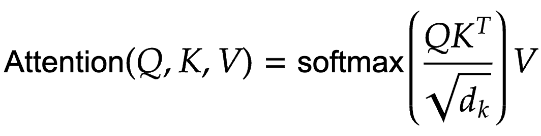
First, the Query and Key matrices are multiplied to arrive at a product term. Let us call this term the  Product. Next, we scale the product term with
  ; this was done to prevent the vanishing gradient problem, as explained in our previous blog post. Finally, the scaled Product term is passed through a softmax layer. The resultant output is multiplied by the value matrix to arrive at the final attention layer.
The entire animation is neatly encapsulated in the attention equation, as shown in Equation 1.
Let’s now talk about a problem with the above module. As we have seen earlier, the attention module can be easily extended to Self-Attention. In a Self-Attention block, the Query, Key, and Value matrices come from the same source.
Intuitively the attention block will attend to each token of the inputs. Take a moment and think about what can possibly go wrong here.
In NMT (Neural Machine Translation), we predict a target token in the decoder given a set of previously decoded target tokens and the input tokens.
If the decoder already has access to all the target tokens (both previous and future), it will not learn to decode. We would need to mask out the target tokens that are not yet decoded by the decoder. This process is necessary to have an auto-regressive decoder.
Vaswani et al. made a minute modification to this attention pipeline to accomplish masking. Before passing the scaled product through a softmax layer, they would mask certain parts of the product with a large number (e.g., negative infinity).
The change is visualized in Video 3 and termed Masked Multi-Head Attention or MMHA.
Video 3: Animation of the Masked-Multi-Head-Attention module.
Connecting Wires
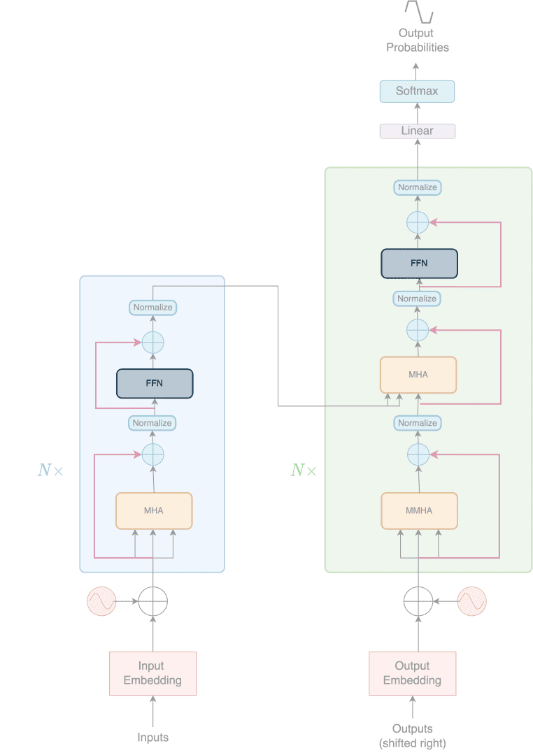
At this point, we have covered the most important building block of the Transformer architecture, attention. But despite what the paper title says (Attention Is All You Need), only attention cannot create the entire model. We need connecting wires to hold each piece together, as shown in Figure 1.
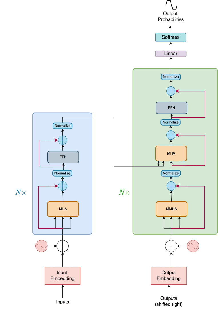
The connecting wires that hold the architecture together are:
- Skip Connection
- Layer Normalization
- Feed-Forward Network
- Positional Encoding
Skip Connections
Intuitively skip connections introduce the representation of a previous stage into a later stage. This allows the raw representation prior to a sub-layer to be injected along with the output from the sub-layer. The skip connections in the Transformers architecture are highlighted with red arrows in Figure 2.
Now, this raises the question, why is it important?
Did you notice that in this blog post series, every time a part of the architecture is mentioned, we bring up the original figure of the entire architecture shown at the very beginning? This is because we process the information better when we reference it with information received at an earlier stage.
Well, it turns out the Transformer works the same way. Creating a mechanism to add representations of past stages into later stages of the architecture allows the model to process the information better.
Layer Normalization
The official TensorFlow documentation of Layer Normalization says:
Notice that with Layer Normalization, the normalization happens across the axes within each example rather than across different examples in the batch.
Here the input is a matrix  with
with  rows where is the number of words in the input sentence. The normalization layer is a row-wise operation that normalizes each row with the same weights.
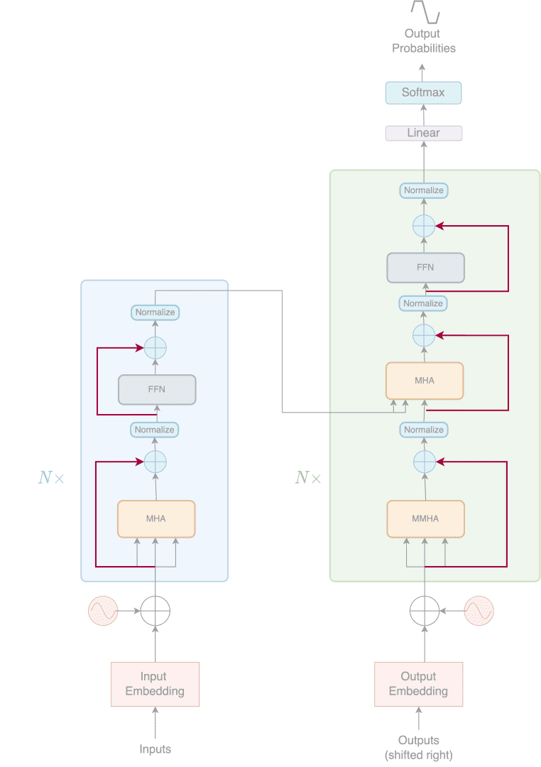
In NLP tasks, as well as in the transformer architecture, the requirement is to be able to calculate the statistics across each feature dimension and instance independently. Thus Layer Normalization makes more intuitive sense than Batch Normalization. The highlighted parts in Figure 3 show the Layer Normalization.

We would also like to bring forward a stack exchange discussion thread about why Layer Normalization works in the Transformer architecture.
Feed-Forward Network
Each encoder and decoder layer consists of a fully connected feed-forward network. The purpose of this layer is straightforward, as shown in Equation 2.
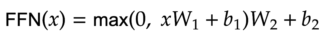
The idea is to project the attention layer output into a higher dimensional space. This essentially means the representations are stretched to a higher dimension, so their details are magnified for the next layer. The application of these layers in the Transformers architecture is shown in Figure 4.
Let us pause here and take a look back at the architecture.
- We studied the encoder and the decoder
- The evolution of attention, as we see in Vaswani et al.
- Skip connections for contextualization
- Layer normalization
- And finally, feed-forward networks
But there is still a part of the entire architecture that is missing. Can we guess what it is from Figure 5?

Positional Encoding
Now, before we understand positional encoding and why it has been introduced in the architecture, let us first look at what our architecture achieves in contrast to sequential models like RNN and LSTM.
The transformer can attend to parts of the input tokens. The encoder and decoder units are built out of these attention blocks, along with non-linear layers, layer normalization, and skip connections.
But RNNs and other sequential models had something that the architecture still lacks. It is to understand the order of the data. So how do we introduce the order of the data?
- We can add attention to a sequential model, but then it will be similar to Bahdanau’s or Luong’s attention which we have already studied. Furthermore, adding a sequential model will beat the purpose of using only attention units for the task at hand.
- We can also inject the data order into the model along with the input and target tokens.
Vaswani et al. opted for the 2nd option. This meant encoding the position of each token and injecting it with the input. So, now there are a couple of ways we can achieve positional encoding.
The first is to simply encode everything in a binary encoding scheme, as shown in Figure 6. Consider the following code snippet where we visualize the binary encoding of a range of numbers.
ncorresponds to the range of0-npositionsdimscorresponds to the dimension to which each position is encoded
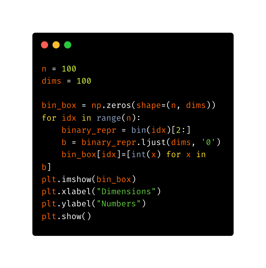
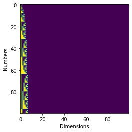
The output of the code snippet in Figure 6 is shown in Figure 7.
Vaswani et al., however, introduced a sine and cosine function that encodes the sequence position according to Equations 3 and 4:
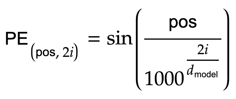
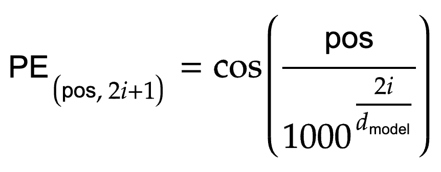
Here, pos refers to the position, and i is the dimension. Figure 8 is the code to implement the equations.

The output of the code in Figure 8 is shown in Figure 9.
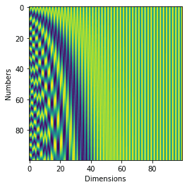
The two encodings look similar, don’t they? Positional encoding is a system in which each position is encoded into a vector. An important thing to note here is that each vector should be unique.
Binary encoding seems to be a perfect candidate for positional encoding. The problem with the binary system is that of 0s. This means binary is discrete in nature. Deep Learning models, on the other hand, love to work with continuous data.
The reason for using sinusoidal encoding is thus three-fold.
- The encoding system is not only dense but also continuous in the range of 0 and 1 (sinusoids are bound in this range).
- It provides a geometric progression, as evident in Figure 10. A geometric progression is easily learnable as it repeats itself after specific intervals. Learning the interval rate and the magnitude will allow any model to learn the pattern itself.
- Vaswani et al. hypothesize that doing this would allow the model to learn relative positions better since any position offset by a value

") can be estimated by a linear function of
can be estimated by a linear function of  .
.

What's next? I recommend PyImageSearch University.
53+ total classes • 57+ hours of on-demand code walkthrough videos • Last updated: Sept 2022
★★★★★ 4.84 (128 Ratings) • 15,800+ Students Enrolled
I strongly believe that if you had the right teacher you could master computer vision and deep learning.
Do you think learning computer vision and deep learning has to be time-consuming, overwhelming, and complicated? Or has to involve complex mathematics and equations? Or requires a degree in computer science?
That’s not the case.
All you need to master computer vision and deep learning is for someone to explain things to you in simple, intuitive terms. And that’s exactly what I do. My mission is to change education and how complex Artificial Intelligence topics are taught.
If you're serious about learning computer vision, your next stop should be PyImageSearch University, the most comprehensive computer vision, deep learning, and OpenCV course online today. Here you’ll learn how to successfully and confidently apply computer vision to your work, research, and projects. Join me in computer vision mastery.
Inside PyImageSearch University you'll find:
- ✓ 53+ courses on essential computer vision, deep learning, and OpenCV topics
- ✓ 53+ Certificates of Completion
- ✓ 57+ hours of on-demand video
- ✓ Brand new courses released regularly, ensuring you can keep up with state-of-the-art techniques
- ✓ Pre-configured Jupyter Notebooks in Google Colab
- ✓ Run all code examples in your web browser — works on Windows, macOS, and Linux (no dev environment configuration required!)
- ✓ Access to centralized code repos for all 450+ tutorials on PyImageSearch
- ✓ Easy one-click downloads for code, datasets, pre-trained models, etc.
- ✓ Access on mobile, laptop, desktop, etc.
Summary
Now at this point, almost everything about transformers is known to us. But it is also important to pause and ponder the necessity of such an architecture.
In 2017, the answer lay in their paper. Vaswani et al. mention their reasons for choosing the simpler version of other transduction models published at the time. But we have come a long way since 2017.
In the last 5 years, transformers have absolutely taken over Deep Learning. There is no task, nook, or corner safe from attention applications. So what made this model so good? And how was that conceptualized in a simple Machine Translation task?
Firstly, Deep Learning researchers are not soothsayers, so there was no way of knowing that Transformers would be so good at every task. But the architecture is intuitively simple. It works by attending to parts of the input tokens that are relevant to parts of the target token. This approach worked wonders for Machine Translation. But will it not work on other tasks? Image Classification, Video Classification, Text-to-Image generation, segmentation, or volume rendering?
Anything that can be expressed as tokenized input being mapped to a tokenized output set falls in the realm of Transformers.
This brings the theory of Transformers to an end. In the next part of this series, we will focus on creating this architecture in TensorFlow and Keras.
Citation Information
A. R. Gosthipaty and R. Raha. “A Deep Dive into Transformers with TensorFlow and Keras: Part 2,” PyImageSearch, P. Chugh, S. Huot, K. Kidriavsteva, and A. Thanki, eds., 2022, https://pyimg.co/pzu1j
@incollection{ARG-RR_2022_DDTFK2,
  author = {Aritra Roy Gosthipaty and Ritwik Raha},
  title = {A Deep Dive into Transformers with {TensorFlow} and {K}eras: Part 2},
  booktitle = {PyImageSearch},
  editor = {Puneet Chugh and Susan Huot and Kseniia Kidriavsteva and Abhishek Thanki},
  year = {2022},
  note = {https://pyimg.co/pzu1j},
}
Want free GPU credits to train models?
- We used Jarvislabs.ai, a GPU cloud, for all the experiments.
- We are proud to offer PyImageSearch University students $20 worth of Jarvislabs.ai GPU cloud credits. Join PyImageSearch University and claim your $20 credit here.
In Deep Learning, we need to train Neural Networks. These Neural Networks can be trained on a CPU but take a lot of time. Moreover, sometimes these networks do not even fit (run) on a CPU.
To overcome this problem, we use GPUs. The problem is these GPUs are expensive and become outdated quickly.
GPUs are great because they take your Neural Network and train it quickly. The problem is that GPUs are expensive, so you don’t want to buy one and use it only occasionally. Cloud GPUs let you use a GPU and only pay for the time you are running the GPU. It’s a brilliant idea that saves you money.
JarvisLabs provides the best-in-class GPUs, and PyImageSearch University students get between 10-50 hours on a world-class GPU (time depends on the specific GPU you select).
This gives you a chance to test-drive a monstrously powerful GPU on any of our tutorials in a jiffy. So join PyImageSearch University today and try it for yourself.

Join the PyImageSearch Newsletter and Grab My FREE 17-page Resource Guide PDF
Enter your email address below to join the PyImageSearch Newsletter and download my FREE 17-page Resource Guide PDF on Computer Vision, OpenCV, and Deep Learning.
The post A Deep Dive into Transformers with TensorFlow and Keras: Part 2 appeared first on PyImageSearch.
September 26, 2022 at 06:30PM
Click here for more details...
=============================
The original post is available in PyImageSearch by Aritra Roy Gosthipaty and Ritwik Raha
this post has been published as it is through automation. Automation script brings all the top bloggers post under a single umbrella.
The purpose of this blog, Follow the top Salesforce bloggers and collect all blogs in a single place through automation.
============================


Post a Comment