Partial Derivatives and Jacobian Matrix in Stochastic Gradient Descent : Puneet Mangla
by: Puneet Mangla
blow post content copied from PyImageSearch
click here to view original post
Table of Contents
Partial Derivatives and Jacobian Matrix in Stochastic Gradient Descent
Vector calculus is a cornerstone of modern machine learning and optimization, providing the mathematical tools necessary to navigate and manipulate functions in multi-dimensional spaces. At its core, vector calculus deals with vector fields and operations on vectors, which are essential for understanding how changes in input variables affect the output of complex models.
This branch of mathematics is particularly important in the context of optimization algorithms, which are used to fine-tune machine learning models to achieve the best possible performance. In this blog post, we will focus on two critical concepts within vector calculus: partial derivatives and the Jacobian matrix.
These concepts are not only fundamental to the theory of optimization but also play a pivotal role in practical applications, especially in the widely used Stochastic Gradient Descent (SGD) algorithm. By exploring these topics, we aim to provide a comprehensive understanding of how vector calculus underpins the optimization processes that drive the success of machine learning models.
This lesson is the 1st of a 2-part series on Vector Calculus:
- Partial Derivatives and Jacobian Matrix in Stochastic Gradient Descent (this tutorial)
- Hessian Matrix, Taylor Series, and the Newton-Raphson Method
To learn how to implement stochastic gradient descent using the concepts of vector calculus, just keep reading.
Basics of Vector Calculus
Vector calculus is crucial for understanding and optimizing functions in machine learning. It provides the tools needed to analyze how changes in input variables affect the output of a model. This is particularly important in optimization algorithms like Stochastic Gradient Descent (SGD), where the goal is to minimize a loss function by adjusting model parameters. By using partial derivatives and the Jacobian matrix, we can efficiently compute the gradients needed to update the parameters and improve the model’s performance. Understanding vector calculus is, therefore, essential for anyone working in the field of machine learning and optimization.
Vectors
A vector is a mathematical object that has both magnitude and direction. In the context of vector calculus, vectors are used to represent quantities that have multiple components. For example, a vector in 3-dimensional space can be written as:

where  ,
,  , and
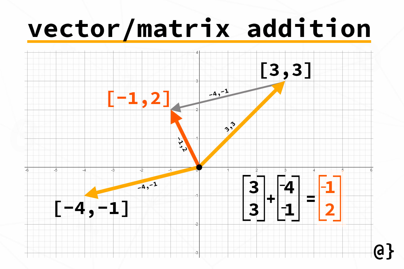
, and  are the components of the vector. The vectors can be added together and multiplied by scalars, which are single numbers. The operations on vectors follow specific rules (Figure 1), such as the following:
- Vector Addition:

- Vector Subtraction:

- Scalar Multiplication:

Differentiation of Univariate Functions
What Are Derivatives?
Univariate functions are those of a single variable. They are the simplest type of functions and are often used to introduce the basic concepts of calculus. A univariate function can be written as:
")
where  is the input variable.
For example, the position of a car is given by a univariate function  = (t+2)(t-6)") , where
, where  is time in seconds. In order to calculate the velocity
 ") of the car at any time , we need to compute the instantaneous rate of change of position
of the car at any time , we need to compute the instantaneous rate of change of position ") with respect to time . This is where derivatives come in handy.
with respect to time . This is where derivatives come in handy.
Given a univariate function , the derivative }/{dx}") or
or ") represents the instantaneous rate of change (or instantaneous slope) of the function
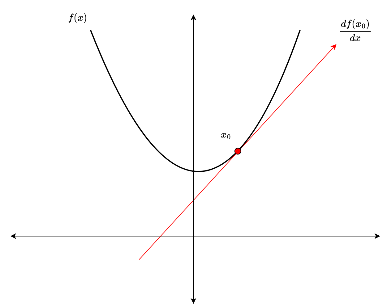
represents the instantaneous rate of change (or instantaneous slope) of the function  with respect to . Mathematically, the derivative (Figure 2) of a function at a point is calculated as follows:
 = \displaystyle\frac{df(x)}{dx} = \lim_{h \rightarrow 0} \displaystyle\frac{f(x+h) - f(x)}{h}") .
.
If the derivative  \leq 0") , it means the function is decreasing at that point. Otherwise, it is nondecreasing.
, it means the function is decreasing at that point. Otherwise, it is nondecreasing.
For example, the derivative of  = x^2") is:
is:
 = \displaystyle\frac{df(x)}{dx} = \displaystyle\frac{d}{dx} (x^2) = 2x")
This derivative tells us the rate at which changes with respect to .
Derivatives of Common Functions
The following are the derivatives of some common functions:
- Constant function: If
 = \text{c}") , where
, where  is a constant, then
  = 0") .
. - Polynomial function: If
 = x^n") , where
, where  is the degree of the polynomial, then
  = n \cdot x^{n-1}") .
. - Logarithmic function: If
 = \ln(x)") , then
, then  = 1/x") .
. - Exponential functions: If
 = e^x") , then
, then  = e^x") . However, if
. However, if  = a^x") , where
, where  is a constant, then
  = a^x \cdot \ln(a)") .
. - Trigonometric functions:
- If
 = \sin(x)") , then
, then  = \cos(x)") .
. - If
 = \cos(x)") , then
, then  = -\sin(x)") .
. - If
 = \tan(x)") , then
, then  = \sec^2(x)") .
.
- If
Central Difference Formula
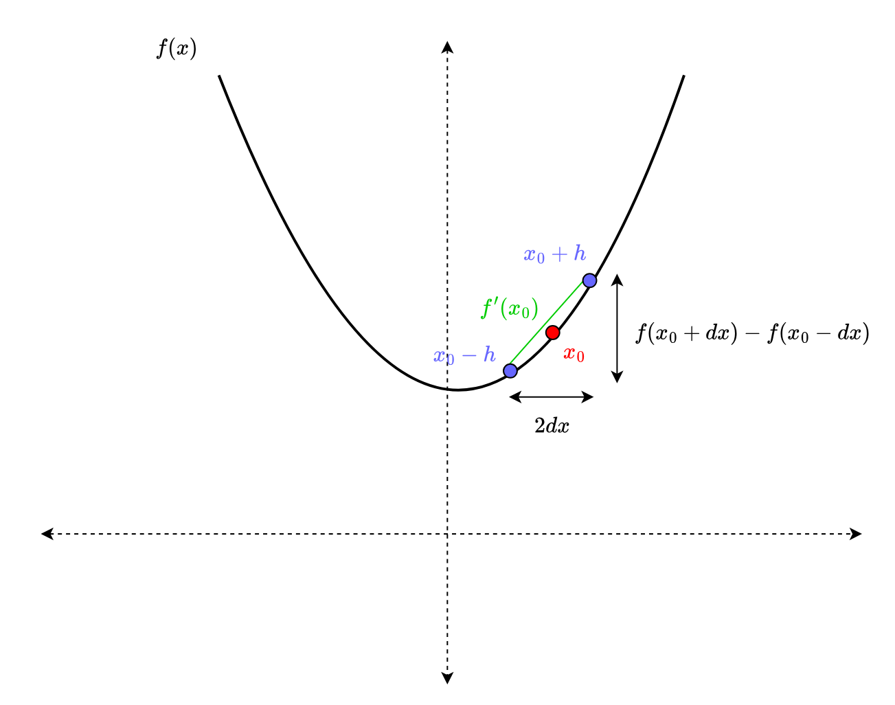
To numerically estimate the derivative of a function at a point , SciPy and other numerical packages employ the central difference formula (Figure 3) as follows:
 = \lim_{h \rightarrow 0} \displaystyle\frac{f(x+h) - f(x)}{h} \approx\displaystyle\frac{f(x + dx) - f(x- dx)}{2 dx}")
where  is a parameter that is usually kept very small (the smaller, the better). In easier terms, the central difference formula approximates the derivative using the function value in the small neighborhood of the point .
The following code snippet shows how to compute derivatives of univariate functions using the SciPy package. If you don’t have SciPy installed in your system, you can do so via pip install scipy.
import numpy as np
import matplotlib.pyplot as plt
from scipy.misc import derivative
import warnings
warnings.filterwarnings("ignore")

# objective function
def objective(x):
 return (x+2)*(x-6)

x0 = 5 # calculate the instantaneous velocity at this point.
y0 = objective(x0)
dfy = derivative(objective, x0, dx=1e-6) # calculate derivative using SciPY package
In this code, we first import the necessary libraries: NumPy for numerical operations, Matplotlib for plotting, and SciPy for calculating derivatives (Lines 1-5). We then define an objective function  = (x + 2)(x - 6)") (Lines 8 and 9). At the point
(Lines 8 and 9). At the point  , we calculate the function value
  and the derivative (slope) at this point using SciPy’s
 derivative function (Lines 11-13). The derivative is printed and plotted to show the instantaneous rate of change at  (Figure 4).
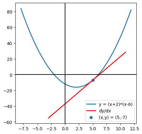
print('dy/dx at x = %.3f is %.3f' % (x0, dfy))

# plot the curve for graphic visualization
plt.figure(figsize=(5,5))
plt.rcParams.update({'font.size': 10})
xs = np.arange(-8, 12, 0.1)
plt.plot(xs, objective(xs), linewidth=2, label='y = (x+2)*(x-6)')

# plot the tangent touching the point x0 and having slope dy/dx
tangent_fn = lambda x: dfy*x + (y0 - dfy*x0)
xs = np.arange(-3, 11, 0.1)
plt.plot(xs, tangent_fn(xs), linewidth=2, ls='-', color='red', label='dy/dx')

# plot (x0, y0),  x and y axis
plt.scatter(x0, y0, label='(x,y) = ({},{})'.format(x0, y0))
plt.axhline(y=0, ls='-', color='black')
plt.axvline(x=0, ls='-', color='black')
plt.legend()
plt.show()
Output:
dy/dx at x = 5.000 is 6.000
Partial Derivatives and Gradients
Multivariate Functions
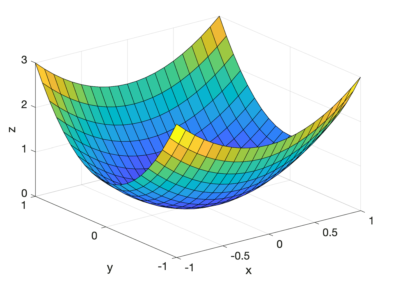
Multivariate functions (Figure 5) are functions of multiple variables. These functions are more complex and are used to model systems with multiple inputs (e.g., machine learning models such as linear and logistic regressions). A multivariate function can be written as:
")
where ( ) are the
  input variables that can also be represented as an -dimensional vector:

For example, the volume of a cylinder  = \pi x_1^2x_2") is a multivariate function in
is a multivariate function in  -dimensional space
  because it takes two inputs: the radius
  and the height
  of the cylinder.
For multivariate functions  = f(x_1, x_2, \dotsc, x_m)") , where the input
, where the input  is an -dimensional vector, the generalization of the derivative is known as the gradient.
The gradient is a collection of quantities known as partial derivatives.
Partial Derivatives
Partial derivatives are useful for multivariate functions (e.g., the volume of a cylinder), because they can help us understand how the volume changes when one of the variables (radius or height) changes while the other is fixed.
The partial gradient of the function with respect to a variable  (e.g., radius) is obtained by varying only that variable and keeping others (e.g., height) constant. In other words,
}{\partial x_i} = \lim_{h \rightarrow 0} \displaystyle\frac{f(x_1, x_i + h, \dotsc, x_m) - f(x)}{h}")
Gradients, aka Jacobian of Multivariate Functions
The gradient  the function (aka Jacobian or Jacobian matrix) with respect to is then represented as an -dimensional row vector as follows:
![\nabla_x f = \left [ \displaystyle\frac{\partial f(x)}{\partial x_1}, \displaystyle\frac{\partial f(x)}{\partial x_2},\dotsc, \displaystyle\frac{\partial f(x)}{\partial x_m} \right ] \in \mathbb{R}^{1 \times m}](https://b2633864.smushcdn.com/2633864/wp-content/latex/996/996790705f17d87181d071cacfd5cee4-ffffff-000000-0.png?lossy=2&strip=1&webp=1 "\nabla_x f = \left [ \displaystyle\frac{\partial f(x)}{\partial x_1}, \displaystyle\frac{\partial f(x)}{\partial x_2},\dotsc, \displaystyle\frac{\partial f(x)}{\partial x_m} \right ] \in \mathbb{R}^{1 \times m}")
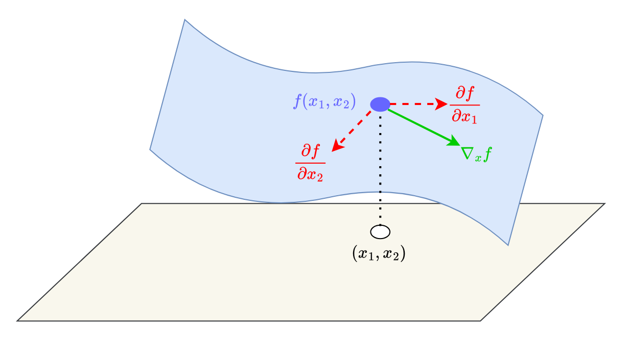
The gradient vector ^T") represents the direction of the steepest ascent (Figure 6), that is, the maximum increase in function value . This important property is the basis of all gradient-based optimization algorithms in machine learning (as we will see later in this post).
represents the direction of the steepest ascent (Figure 6), that is, the maximum increase in function value . This important property is the basis of all gradient-based optimization algorithms in machine learning (as we will see later in this post).
The following code snippet shows how to compute gradients of multivariate functions using the concepts of partial derivatives with SciPy.
import numpy as np
from scipy.misc import derivative
import matplotlib.pyplot as plt

# objective function
def objective(x1, x2):
 return (x1+2)*(x1-5) + (x2+1)*(x2-3)
In this code, we start by importing the necessary libraries: NumPy for numerical operations, SciPy for calculating derivatives, and Matplotlib for plotting (Lines 34-36). We define a multivariate objective function ") in 2 dimensions (Lines 39 and 40).
in 2 dimensions (Lines 39 and 40).
x1_0, x2_0 = -3, -2
f = objective(x1_0, x2_0)

df_x1 = derivative(lambda x1: objective(x1, x2_0), x1_0, dx=1e-6)
df_x2 = derivative(lambda x2: objective(x1_0, x2), x2_0, dx=1e-6)
We then set initial values for and and calculate the function value at these points (Lines 42 and 43). To find the partial derivatives, we use the derivative function from SciPy by holding one variable constant and differentiating with respect to the other (Lines 45 and 46). We print and plot the gradient, which consists of the partial derivatives with respect to and (Figure 7).
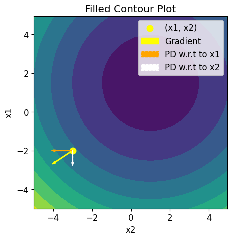
print("Gradient of f(x) at x = (%.3f, %.3f) is (%.3f, %.3f)"% (x1_0, x2_0, df_x1, df_x2))

# plot the curve for graphic visualization
plt.figure(figsize=(5,5))
plt.rcParams.update({'font.size': 12})
x1s, x2s = np.arange(-5.0, 5.0, 0.05), np.arange(-5.0, 5.0, 0.05)
zs = [[objective(x1,x2) for x2 in x2s] for x1 in x1s]
plt.contourf(x2s, x1s, zs)
plt.title('Filled Contour Plot')
plt.xlabel('x2')
plt.ylabel('x1')

p1 = plt.scatter(x1_0, x2_0, color='yellow', linewidths=4, label='(x1, x2)')
a1 = plt.arrow(x1_0, x2_0, 0.1*df_x1, 0.1*df_x2, color='yellow', width=0.04, label='Gradient')
a2 = plt.arrow(x1_0, x2_0, 0.1*df_x1, 0, color='orange', width=0.04, ls='--', label='PD w.r.t to x1')
a3 = plt.arrow(x1_0, x2_0, 0, 0.1*df_x2, color='white', width=0.04, ls='--', label='PD w.r.t to x2')
plt.legend([p1, a1, a2, a3,], ['(x1, x2)', 'Gradient', 'PD w.r.t to x1', 'PD w.r.t to x2',])
plt.show()
Output:
Gradient of f(x) at x = (-3.000, -2.000) is (-9.000, -6.000)
Application of Derivatives and Gradients in Stochastic Gradient Descent
Stochastic Gradient Descent (SGD) is a powerful optimization algorithm widely used in machine learning to minimize loss functions and improve model performance. The core idea behind SGD is to iteratively update model parameters in the direction that reduces the loss function.
Gradients play a critical role in SGD by providing the direction and magnitude of the updates needed to minimize the loss function. By iteratively adjusting the model parameters in the direction of the negative gradient, SGD efficiently navigates the loss landscape to find the optimal parameters.
This process allows machine learning models to learn from data and improve their performance over time. Understanding the application of derivatives and gradients in SGD is essential for effectively implementing and tuning optimization algorithms in machine learning.
Let’s explore how these mathematical tools are applied in SGD.
Weight Updates in Stochastic Gradient Descent
Consider the scenario where we want to create a model that predicts whether an individual has diabetes or not. This is a case of binary classification, and let’s assume that  represents the collection or dataset of
  -dimensional inputs (e.g., age, weight, height, cholesterol, etc.), for
  patients.
Further, let’s assume that

where  denotes their corresponding ground truth binary labels (
1 means diabetes, and 0 means no diabetes). The prediction  of a logistic regression model is given as follows:
")
where  denotes the weights of the logistic regression model and
 = \displaystyle\frac{1}{1 + \exp(-x)}")
is the sigmoid function that squashes any real value in the range ") .
.
The logistic regression minimizes the binary cross-entropy loss between the predicted and the ground-truth label  to find the optimal parameters
  .
.
 = \displaystyle\sum_{i=1}^N L(x_i, y_i, \beta)")
where
 & = & -y_i \log(\hat{y_i}) - (1-y_i)\log(1- \hat{y_i})\vspace{5pt}\\ & = & -y_i \log(\sigma(x_i^T\beta)) - (1-y_i)\log(1- \sigma(x_i^T\beta))\end{array}")
is loss function for one data point ") .
.
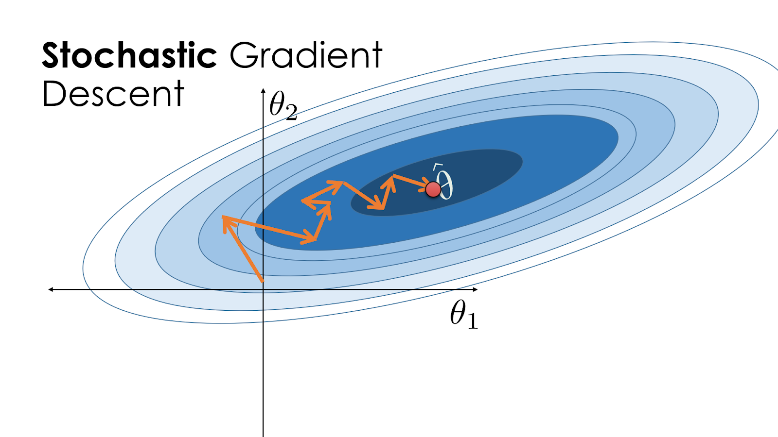
To minimize the loss function, Stochastic Gradient Descent (Figure 8) iteratively updates the parameters  in the direction of the negative gradient of the loss function. We will start by randomly initializing its parameters to
  and then subsequently updating the model parameters via the following gradient descent rule:
)^T")
where:
 is the parameter vector at iteration
  is the learning rate, a hyperparameter that controls the step size of the updates
 = -y_t \cdot x_t + \hat{y}_t \cdot x_t") is the gradient of the loss function with respect to model parameter based on a random data point
is the gradient of the loss function with respect to model parameter based on a random data point ") sampled from the dataset.
sampled from the dataset.
The learning rate is crucial for the convergence of SGD. If is too large, the updates may overshoot the minimum, leading to divergence. If is too small, the convergence may be very slow.
Implementation of Stochastic Gradient Descent
import numpy as np
import matplotlib.pyplot as plt

# sigmoid function
def sigmoid(x):
     return 1/(1+ np.exp(-x))

# objective function
def objective(X, Y, beta):
     Y_pred = sigmoid(X @ beta)
     loss = -Y*np.log(Y_pred) - (1-Y)*np.log(1-Y_pred)
     return loss.mean()
In this code, we implement a logistic regression model from scratch. We begin by defining a sigmoid function and an objective function to calculate the loss (Lines 70-77). The objective function uses the sigmoid function to predict  and calculates the mean binary cross-entropy loss.
# generate ground-truth labels
def get_gt_labels(X):
     p = np.array([1, -1])
     Y = X @ p
     return (Y >=0).astype(np.float32)

# Creating a sample logistic regression dataset
N = 2000 # Total size of dataset
X = np.random.uniform(low=[-1.0, -1.0], high=[1.0, 1.0], size=(N, 2)) # Input data
Y = get_gt_labels(X) # ground-truth labels

alpha = 2 # step size
T = 500 # total iterations
beta = np.random.uniform(-10.0, 10.0, X.shape[1]) # randomly initialize parameters
path = [beta]
Next, we define a function to generate ground-truth labels for our input data (Lines 80-83) and use it to create a sample logistic regression dataset with 2000 data points, where  is the input data, and are the ground-truth labels (Lines 86-88). We initialize parameters for gradient descent, including step size and total iterations
  , and randomly initialize the weights (Lines 90-93).
for t in range(T):
     index = np.random.choice(range(N))
     x_t, y_t = X[index, :], Y[index] # randomly sample an example from dataset

     y_hat_t = sigmoid(x_t @ beta)
     gradient = -x_t*y_t + x_t*y_hat_t # compute gradient
     beta = beta - alpha*gradient # perform gradient descent

     if (t+1)%50 == 0 or (t==T-1):
          path.append(beta)
We then perform stochastic gradient descent by iterating over the dataset for iterations (Lines 95-104). In each iteration, we randomly sample a data point, compute the gradient of the loss with respect to the weights, and update the weights accordingly.
print("Beta Estimated  = {}".format(np.round_(beta, 3)))

Y_hat = sigmoid(X @ beta)
print("Loss = {}".format(objective(X, Y, beta)))

Y_hat_binary = (Y_hat >=0.5).astype(np.float32)
accuracy = (Y_hat_binary == Y).mean()

print("Accuracy = {}".format(accuracy))


# plot the curve for graphic visualization
plt.figure(figsize=(5,5))
plt.rcParams.update({'font.size': 12})

b1s, b2s = np.arange(-15.0, 15.0, 0.5), np.arange(-15.0, 15.0, 0.5)
zs = [[objective(X, Y, np.array([b1, b2])) for b2 in b2s] for b1 in b1s]
plt.contourf(b1s, b2s, zs) # Visualize the contour plot

plt.title('Filled Contour Plot')
plt.xlabel('beta[1]')
plt.ylabel('beta[0]')

# visualize the optimal point
plt.scatter(beta[1], beta[0], linewidth=6, color='orange', label='optimum beta, Loss = {:.2f}'.format(objective(X, Y, beta)))

for i in range(len(path) -1):
     plt.arrow(path[i][1], path[i][0], (path[i+1][1] -path[i][1]), (path[i+1][0] - path[i][0]), color='yellow', width=0.03)

plt.legend()
plt.show()
Output:
Beta Estimated  = [ 10.997 -10.379]
Loss = 0.07611120384902355
Accuracy = 0.987
We store the path of values for visualization. After the iterations, we print the estimated weights, compute the predicted labels, calculate the loss, and determine the accuracy of the model (Lines 106-114). Finally, we visualize the objective function’s contour plot and the optimization path taken by the gradient descent algorithm (Figure 9). This visualization helps us understand how the weights converge to the optimal solution, minimizing the loss function.
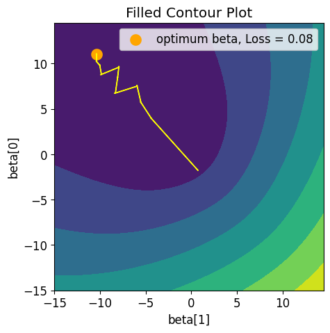
From the output of the code, we can see that the stochastic gradient descent algorithm converged to optimal model parameters, which provided us with an accuracy of 98.7% on the sample dataset.
What's next? We recommend PyImageSearch University.
86+ total classes • 115+ hours hours of on-demand code walkthrough videos • Last updated: March 2025
★★★★★ 4.84 (128 Ratings) • 16,000+ Students Enrolled
I strongly believe that if you had the right teacher you could master computer vision and deep learning.
Do you think learning computer vision and deep learning has to be time-consuming, overwhelming, and complicated? Or has to involve complex mathematics and equations? Or requires a degree in computer science?
That’s not the case.
All you need to master computer vision and deep learning is for someone to explain things to you in simple, intuitive terms. And that’s exactly what I do. My mission is to change education and how complex Artificial Intelligence topics are taught.
If you're serious about learning computer vision, your next stop should be PyImageSearch University, the most comprehensive computer vision, deep learning, and OpenCV course online today. Here you’ll learn how to successfully and confidently apply computer vision to your work, research, and projects. Join me in computer vision mastery.
Inside PyImageSearch University you'll find:
- ✓ 86+ courses on essential computer vision, deep learning, and OpenCV topics
- ✓ 86 Certificates of Completion
- ✓ 115+ hours hours of on-demand video
- ✓ Brand new courses released regularly, ensuring you can keep up with state-of-the-art techniques
- ✓ Pre-configured Jupyter Notebooks in Google Colab
- ✓ Run all code examples in your web browser — works on Windows, macOS, and Linux (no dev environment configuration required!)
- ✓ Access to centralized code repos for all 540+ tutorials on PyImageSearch
- ✓ Easy one-click downloads for code, datasets, pre-trained models, etc.
- ✓ Access on mobile, laptop, desktop, etc.
Summary
In this blog post, we delve into the essential concepts of vector calculus, focusing on vectors, differentiation of univariate functions, and understanding derivatives. We begin with the basics, exploring what vectors are and how they function in mathematical contexts. Then, we discuss the differentiation of univariate functions, defining derivatives and examining their properties, including common functions and the center difference formula.
Next, we extend our exploration to multivariate functions, introducing partial derivatives and gradients, which are key to understanding the Jacobian matrix. We explain how partial derivatives provide a way to differentiate functions with multiple variables and how gradients, or Jacobians, play a crucial role in optimizing such functions. This section equips us with the tools needed to tackle complex problems involving multiple variables.
Finally, we apply these concepts to stochastic gradient descent (SGD), a fundamental optimization technique in machine learning. We detail how derivatives and gradients are used to update weights in SGD, ensuring the model learns efficiently from data. The implementation of SGD is covered, demonstrating how these mathematical principles translate into practical algorithms for training machine learning models. This comprehensive guide provides a thorough understanding of the mathematical foundations and their applications in modern optimization techniques.
Citation Information
Mangla, P. “Partial Derivatives and Jacobian Matrix in Stochastic Gradient Descent,” PyImageSearch, P. Chugh, S. Huot, and P. Thakur, eds., 2025, https://pyimg.co/1wh34
@incollection{Mangla_2025_partial-derivatives-jacobian-matrix-stochastic-gradient-descent,
  author = {Puneet Mangla},
  title = ,
  booktitle = {PyImageSearch},
  editor = {Puneet Chugh and Susan Huot and Piyush Thakur},
  year = {2025},
  url = {https://pyimg.co/1wh34},
}
To download the source code to this post (and be notified when future tutorials are published here on PyImageSearch), simply enter your email address in the form below!

Download the Source Code and FREE 17-page Resource Guide
Enter your email address below to get a .zip of the code and a FREE 17-page Resource Guide on Computer Vision, OpenCV, and Deep Learning. Inside you'll find my hand-picked tutorials, books, courses, and libraries to help you master CV and DL!
The post Partial Derivatives and Jacobian Matrix in Stochastic Gradient Descent appeared first on PyImageSearch.
March 03, 2025 at 07:30PM
Click here for more details...
=============================
The original post is available in PyImageSearch by Puneet Mangla
this post has been published as it is through automation. Automation script brings all the top bloggers post under a single umbrella.
The purpose of this blog, Follow the top Salesforce bloggers and collect all blogs in a single place through automation.
============================


Post a Comment